I. I. Kopach Theory of metallurgical processes - file n1.doc
Federal Agency for Education
GOU VPO "Ural State Technical University- UPI "
A.M. Panfilov
Educational electronic text edition
Prepared by the Department of Theory of Metallurgical Processes
Scientific editor: prof., Doct. chem. M.A. Spiridonov
Methodical instructions for laboratory work in the disciplines "Physicochemistry of metallurgical systems and processes", "Theory of metallurgical processes" for students of all forms of training in metallurgical specialties.
The rules for organizing work in the workshop "Theory of metallurgical processes" of the Department of TMP (specialized audience
MT-431 named after O.A. Esina). The methodology and procedure for performing laboratory work are described, requirements for the content and preparation of reports on laboratory work in accordance with the current GOST and recommendations for their implementation are given.
© GOU VPO USTU-UPI, 2008
Yekaterinburg
Introduction ................................................. .................................................. .................................................. . 4
1 Organization of work in a laboratory workshop on the theory of metallurgical processes ............. 4
1.1 Preparation for laboratory work.................................................. ............................................... 5 1.2 Recommendations on processing measurement results and preparing a report .............................. 5
1.3.1 Construction of graphs ............................................. .................................................. ................... 5
1.3.2 Smoothing experimental data ............................................ ................................... 7
1.3.5 Numerical differentiation of a function given by a set of discrete points ................ 8
approximating some data set .............................................. .................................. 9
1.3.7 Presentation of results ............................................. .................................................. ....... 10
2 Description of laboratory work .............................................. .................................................. ............. eleven
2.1 Study of the kinetics of high-temperature oxidation of iron (Work No. 13) ......................... 12
2.1.1 General regularities of iron oxidation ........................................... .................................. 12 2.1.2 Description of the installation and the procedure for carrying out experiments ... .................................................. ..... 14
2.1.3 Processing and presentation of measurement results .......................................... ................... 15
Control questions................................................ .................................................. ..................... 17
2.2 Study of the temperature dependence of the electrical conductivity of oxide melts
(Work No. 14) ............................................. .................................................. .......................................... nineteen
2.2.1 General information on the nature of electrical conductivity of slags ...................................... 19
2.2.2 Description of the installation and measurement procedure .......................................... ................................ 21
2.2.3 The order of performance of work ............................................ .................................................. ..... 23
2.2.4 Processing and presentation of measurement results .......................................... ................... 24
Control questions................................................ .................................................. ..................... 25
2.3 Study of the kinetics of metal desulfurization by slag on a simulation model (Work No.
15) ............................................................................................................................................................ 26
2.3.1 General information on the kinetics of metal desulfurization by slag ........................................ ..... 26
2.3.2 Mathematical model of the process ............................................ ............................................... 29
2.3.3 The order of work ............................................ .................................................. ...... thirty
2.3.4 Processing and presentation of measurement results .......................................... ................... 31
Control questions................................................ .................................................. ..................... 32
2.4 Thermographic study of the processes of dissociation of natural carbonates (Work No. 16) 33
2.4.1 General regularities of carbonate dissociation ........................................... ...................... 33
2.4.2 Installation diagram and work procedure ......................................... ......................... 39
2.4.3 Processing and presentation of measurement results .......................................... ................... 39
Control questions................................................ .................................................. ..................... 41
2.5 Study of the temperature dependence of the viscosity of oxide melts (Work No. 17) ............. 42
2.5.1 The nature of the viscous resistance of oxide melts .......................................... ................ 42
2.5.2 Description of the installation and the procedure for measuring the viscosity ......................................... .................. 43
2.5.3 The order of work ............................................ .................................................. ...... 45
2.5.4 Processing and presentation of measurement results .......................................... ................... 45 Test questions ............................ .................................................. ......................................... 46
2.6 Reduction of manganese from oxide melt to steel (Work No. 18)
2.6.1 General laws of the electrochemical interaction of metal and slag ............... 47
2.6.2 Process model ............................................. .................................................. ........................ 49
2.6.3 The order of work ............................................ .................................................. ...... 50
Control questions................................................ .................................................. ..................... 52 References .......................... .................................................. .................................................. ..... 53
| STP USTU-UPI 1-96 |
Enterprise standard. General requirements and the rules for the design of diploma and course projects (works). |
| GOST R 1.5-2002 |
GSS. Standards. General requirements for construction, presentation, design, content and designation. |
| GOST 2.105-95 |
ESKD. General requirements for text documents. |
| GOST 2.106-96 |
ESKD. Text documents. |
| GOST 6.30 2003 |
USD. Unified system of organizational and administrative documentation. Requirements for paperwork. |
| GOST 7.32-2001 |
SIBID. Research report. |
| GOST 7.54-88 |
SIBID. Representation of numerical data on the properties of substances and materials in scientific and technical documents. General requirements. |
| GOST 8.417-2002 |
GSOEE. Units of quantities |
Abbreviations and abbreviations
| State standard former USSR or interstate standard (currently). |
|
| Standard adopted The State Committee Of the Russian Federation for Standardization and Metrology (Gosstandart of Russia) or the State Committee of the Russian Federation for Housing and Construction Policy (Gosstroy of Russia). |
|
| State system standardization. |
|
| State system for ensuring the uniformity of measurements. |
|
| Information Technology |
|
| Least square method |
|
| Personal Computer |
|
| Enterprise standard |
|
| Theory of metallurgical processes |
Introduction
Performing laboratory work to study the properties in the metal-slag system and the processes occurring in metallurgical units, allows you to better understand the capabilities of the physicochemical method of analysis and gain skills in its practical application. Additionally, the student gets acquainted with the implementation of some methods of experimental and model research of individual physical and chemical properties and metallurgical processes in general, acquires the skills of processing, analysis and presentation of experimental information.
1 Organization of work in a laboratory workshop on the theory of metallurgical processes
In a laboratory workshop on the theory of metallurgical processes, the main thing is the computer collection of experimental information. This determines a number of features of the organization of work:
Each student receives individual task, performs the experiment in its entirety or a specified part of it and processes the information received. The result of the work includes the obtained numerical characteristics of the phenomenon under study and errors in their determination, graphs illustrating the identified features, and conclusions obtained from the entire set of information. The discrepancy between the quantitative results of work, given in student reports, in comparison with the control marks should not exceed 5%.
The main options for presenting the results are processing experimental data, plotting graphs and formulating conclusions in Microsoft.Excel or OpenOffice.Calc spreadsheets.
With the permission of the teacher, it is temporarily allowed to present a handwritten report with the necessary illustrations and graphs made on graph paper.
The report on the laboratory work performed is sent to the teacher leading the laboratory practice no later than on the working day preceding the next laboratory work. Transfer order (by e-mail, during a break, any teacher or laboratory assistant leading the class at the moment) is determined by the teacher.
Students who have not submitted a report on previous work in time and have not passed the colloquium (testing) are not allowed to the next laboratory work.
Only students who have undergone an introductory briefing on safe work measures in a laboratory practice and signed the instruction sheet are allowed to perform laboratory work.
Work with heating and measuring electrical devices, with chemical glassware and reagents is carried out in accordance with the safety instructions in the laboratory.
After completing the work, the student tidies up the workplace and hands it over to the laboratory assistant.
1.1 Preparation for laboratory work
The main sources in preparation for the lesson are this manual, textbooks and teaching aids recommended by the lecturer, lecture notes.
Preparing for laboratory work, the student during the week preceding the lesson must read and understand the material related to the phenomenon under study, understand the diagrams given in the manual in the design of the installation and the measurement technique and the processing of their results. If difficulties arise, it is necessary to use the recommended literature and consultations of the lecturer and teachers conducting laboratory studies.
The student's readiness to perform the work is controlled by the teacher through an individual survey of each student, or by conducting computer testing. An insufficiently prepared student is obliged to study the material related to this work during the lesson, and to perform the experimental part of the work in an additional lesson after re-checking. The time and procedure for conducting repeated classes is regulated by a special schedule.
1.2 Recommendations for processing measurement results and preparing a report
According to GOST 7.54-88, experimental numerical data should be presented in the form of titled tables. Sample tables are provided for each lab.
When processing the measurement results, it is necessary to use statistical processing: apply smoothing of experimental data, use the least squares method when evaluating the parameters of dependences, etc. and it is imperative to evaluate the error of the obtained values. Special statistical functions are provided in spreadsheets to perform this processing. The necessary set of functions is also available in calculators designed for scientific (engineering) calculations.
1.3.1 Plotting
When performing experiments, as a rule, the values of several parameters are fixed simultaneously. By analyzing their relationship, one can draw conclusions about the observed phenomenon. The visual representation of numerical data makes it extremely easy to analyze their relationship - which is why graphing is such an important step in working with information. Note that among the fixed parameters there is always at least one independent variable - a value whose value changes by itself (time) or which is set by the experimenter. The rest of the parameters are determined by the values of the independent variables. When building graphs, you should follow some rules:
The value of the independent variable is plotted on the abscissa (horizontal axis) and the value of the function is plotted on the ordinate (vertical axis).
The scales along the axes should be chosen so as to use the area of the graph as informative as possible - so that there are fewer empty areas on which there are no experimental points and lines of functional dependencies. To meet this requirement, you often need to specify a non-zero value at the origin of the coordinate axis. In this case, all experimental results must be presented on the graph.
The values along the axes should, as a rule, be multiples of some integer (1, 2, 4, 5) and be evenly spaced. It is categorically unacceptable to indicate the results of specific measurements on the axes. The scale units you select should not be too small or too large (they should not contain multiple leading or trailing zeros). To ensure this requirement, you should use a scale factor of the form 10 X, which is taken out in the axis designation.
The line of functional dependence should be either straight or smooth curve. It is permissible to connect experimental points with a broken line only at the stage of preliminary analysis.
Many of these requirements will be automatically met when charting with spreadsheets, but usually not all and not fully, so you almost always have to adjust the resulting representation.
Spreadsheets have a special service - Chart Wizard (Main menu: Insert Chart). The simplest way to access it is to first select an area of cells that includes both an argument and a function (several functions), and activate the "Chart Wizard" button on the standard panel with the mouse.
Thus, you will get a draft chart that you still need to work with, since the automatic selection of many of the default chart parameters will most likely not ensure that all requirements are met.
First of all, check the size of the numbers on the axes and the letters in the axis labels and function labels in the legend. It is desirable that the font size be the same everywhere, no less than 10 and no more than 14 points, but you will have to set the value for each label separately. To do this, move the cursor over the object of interest (axis, label, legend) and press the right mouse button. In the context menu that appears, select "Format (element)" and in the new menu on a piece of paper labeled "Font" select the desired value. When formatting the axis, you should additionally look at and, possibly, change the values on the sheets with labels "Scale" and "Number". If you do not understand what changes the proposed choice will lead to, do not be afraid to try any option, because you can always discard the changes made by pressing Ctrl + Z, or by selecting the Main menu item "Edit" - Undo, or by clicking on the button "Undo" on the standard toolbar.
If there are a lot of points, and the spread is small and the line looks smooth enough, then the points can be connected with lines. To do this, move the cursor over a point on the chart and press the right mouse button. In the context menu that appears, select the "Format data series" item. In a new window, on a piece of paper labeled "View", you should select the appropriate color and line thickness, and at the same time check the color, size and shape of the dots. This is how the dependences are constructed that approximate the experimental data. If the approximation is performed by a straight line, then two points on the edges of the range of the argument are sufficient. It is not recommended to use the "smoothed curve" option built into spreadsheets due to the inability to adjust the smoothing parameters.
1.3.2 Smoothing experimental data
The experimental data obtained on high-temperature experimental installations are characterized by a large value of the random measurement error. This is mainly due to electromagnetic interference from the operation of a powerful heating device. Statistical processing of the results can significantly reduce the random error. It is known that for a random variable distributed according to the normal law, the error of the arithmetic mean determined from N values in N½ times less than the error of a single measurement. With a large number of measurements, when it is permissible to assume that the random scatter of data over a small segment significantly exceeds the regular change in the value, an effective smoothing technique is to assign the next value of the measured value to the arithmetic mean calculated from several values in a symmetric interval around it. Mathematically, this is represented by the formula:
 (1.1)
(1.1)
and is very easy to implement in spreadsheets. Here y i is the measurement result, and Y i is the smoothed value used instead.
Experimental data obtained using digital data collection systems are characterized by a random error, the distribution of which differs significantly from the normal law. In this case, it may be more efficient to use the median instead of the arithmetic mean. In this case, the measured value in the middle of the interval is assigned the value of the measured value that turned out to be closest to the arithmetic mean. It would seem that a slight difference in the algorithm can change the result very significantly. For example, in the variant of the median estimate, some experimental results may turn out to be completely unused, most likely exactly those that really are
"Jumping out" values with a particularly large error.
1.3.5 Numerical differentiation of a function given by a set of discrete points
The need for such an operation arises quite often when processing experimental points. For example, by differentiating the dependence of concentration on time, the dependence of the rate of the process on time and on the concentration of the reagent is found, which, in turn, makes it possible to estimate the order of the reaction. The operation of numerical differentiation of a function given by a set of its values ( y) corresponding to the corresponding set of argument values ( x), is based on the approximate replacement of the differential of a function by the ratio of its final change to the final change in the argument:
![]() (1.2)
(1.2)
Numerical differentiation is sensitive to errors caused by inaccuracies in the original data, discarding members of a series, etc., and therefore should be performed with caution. To improve the accuracy of estimating the derivative (), they try to first smooth out the experimental data, at least on a small segment, and only then perform differentiation. As a result, in the simplest case for equidistant nodes (the values of the argument differ from each other by the same value x), the following formulas are obtained: for the derivative in the first ( X 1) point:
 for the derivative at all other points ( x), except for the last one:
for the derivative in the latter ( x) point:
If there are a lot of experimental data and it is permissible to neglect several extreme points, you can use stronger smoothing formulas, for example, by 5 points:
or 7 points:
For an uneven arrangement of nodes, we restrict ourselves to the fact that we recommend using a modified formula (1.3) in the form
![]() (1.8)
(1.8)
and do not calculate the derivative at the start and end points.
Thus, to implement numerical differentiation, you need to place suitable formulas in the cells of a free column. For example, unequally spaced argument values are located in column "A" in cells 2 through 25, and function values are in column "B" in the corresponding cells. The derivative values are supposed to be placed in the "C" column. Then in the cell "C3" you should enter the formula (5) in the form:
= (B4 - B2) / (A4 - A2)
and copy (stretch) to all cells in the range C4: C24.
1.3.6 Determination by the method of least squares of the coefficients of the polynomial,
approximating some data set
When numerical information is presented graphically, it is often necessary to draw a line along the experimental points, revealing the features of the obtained dependence. This is done for a better perception of information and to facilitate further analysis of data that have some scatter due to the measurement error. Often, on the basis of a theoretical analysis of the phenomenon under study, it is known in advance what form this line should have. For example, it is known that the dependence of the rate of a chemical process ( v) from temperature must be exponential, and the exponential exponent represents the inverse temperature in an absolute scale:
 This means that on the graph in coordinates ln v- 1 / T should be a straight line,
whose slope characterizes the activation energy ( E) process. As a rule, several straight lines with different slope can be drawn through the experimental points. In a sense, the best of them will be the straight line with the coefficients determined by the least squares method.
In the general case, the least squares method is used to find the coefficients approximating the dependence y (x 1 , x 2 ,…x n) a polynomial of the form
where b and m 1 …m n Are constant coefficients, and x 1 …x n- a set of independent arguments. That is, in the general case, the method is used to approximate a function of several variables, but it is also applicable to describe a complex function of one variable x... In this case, it is usually believed that
 and the approximating polynomial has the form
When choosing the degree of the approximating polynomial n keep in mind that it must necessarily be less than the number of measured values x and y... In almost all cases, it should be no more than 4, rarely 5.
This method is so important that Excel spreadsheets have at least four options for obtaining the values of the desired coefficients. We recommend using the LINEST () function if you work in Excel spreadsheets with Microsoft Office, or the LINEST () function in OpenOffice Calc spreadsheets. They are presented in the list of statistical functions, belong to the class of so-called matrix functions and in this connection have a number of application features. First, it is entered not into one cell, but directly into a range (rectangular area) of cells, since the function returns multiple values. The size of the area horizontally is determined by the number of coefficients of the approximating polynomial (in this example, there are two of them: ln v 0 and E / R), and vertically from one to five lines can be highlighted, depending on how much statistical information is needed for your analysis.
1.3.7 Presentation of results
In a scientific and technical document, when presenting numerical data, an assessment of their reliability should be given and random and systematic errors should be highlighted. The given data errors should be presented in accordance with GOST 8.207–76.
When statistically processing a group of observation results, the following operations should be performed: exclude known systematic errors from observation results;
Calculate the arithmetic mean of the corrected observation results, taken as the measurement result; calculate the estimate of the standard deviation of the measurement result;
Calculate the confidence limits of the random error (random component of the error) of the measurement result;
Calculate the boundaries of the non-excluded systematic error (non-excluded residuals of the systematic error) of the measurement result; calculate the confidence limits of the error of the measurement result.
To determine the confidence limits of the error of the measurement result, the confidence probability R take equal to 0.95. With a symmetric confidence error, the measurement results are presented in the form:
where is the measurement result, ∆ is the margin of error of the measurement result, R Is the confidence level. The numerical value of the measurement result must end with a digit of the same digit as the value of the error ∆.
2 Description of laboratory work
In the first part of each of the sections devoted to specific laboratory work, information is provided on the composition and structure of phases, the mechanism of processes occurring within a phase or at the boundaries of its interface with neighboring phases, the minimum necessary to understand the essence of the phenomenon studied in the work. If the information given is not enough, you should refer to the lecture notes and the recommended literature. Without understanding the first part of the section, it is impossible to imagine what is happening in the system under study in the course of the work, to formulate and comprehend the conclusions based on the results obtained.
The next part of each section is devoted to the hardware or software implementation of a real installation, or a computer model. It provides information about the hardware used and the algorithms used. Without understanding this section, it is impossible to assess the sources of error and what actions should be taken to minimize their impact.
The last part describes the procedure for performing measurements and processing their results. All these questions are submitted to the colloquium prior to the work, or computer testing.
2.1 Study of the kinetics of high-temperature oxidation of iron (Work No. 13)
2.1.1 General laws of iron oxidation
According to the principle of the sequence of transformations of A.A. Baikov, on the surface of iron during its high-temperature oxidation with atmospheric oxygen, all oxides that are thermodynamically stable under these conditions are formed. At temperatures above 572 ° C, the scale consists of three layers: FeO wustite, Fe 3 O 4 magnetite, Fe 2 O 3 hematite. The wustite layer closest to iron, which is approximately 95% of the entire scale thickness, has p-semiconducting properties. This means that there is a significant concentration of ferrous iron vacancies in the FeO cation sublattice, and electroneutrality is provided due to the appearance of electron "holes", which are ferric iron particles. The anionic sublattice of wustite, consisting of negatively charged О 2– ions, is practically defect-free; the presence of vacancies in the cation sublattice significantly increases the diffusion mobility of Fe 2+ particles through wustite and reduces its protective properties.
The intermediate layer of magnetite is an oxide of stoichiometric composition, which has a low concentration of defects in the crystal lattice and, as a result, has increased protective properties. Its relative thickness is 4% on average.
The outer layer of scale - hematite has n-type conductivity. The presence of oxygen vacancies in the anionic sublattice facilitates the diffusion of oxygen particles through it, in comparison with iron cations. The relative thickness of the Fe 2 O 3 layer does not exceed 1% .
At temperatures below 572 ° C, wustite is thermodynamically unstable; therefore, the scale consists of two layers: magnetite Fe 3 O 4 (90% of the thickness) and hematite Fe 2 O 3 (10%).
The formation of a continuous protective film of scale on the surface of iron leads to its separation from the air atmosphere. Further oxidation of the metal occurs due to the diffusion of reagents through the oxide film. The considered heterogeneous process consists of the following stages: oxygen supply from the volume of the gas phase to the boundary with the oxide by molecular or convective diffusion; adsorption of O2 on the surface of the oxide; ionization of oxygen atoms with the formation of О 2– anions; diffusion of oxygen anions in the oxide phase to the interface with the metal; ionization of iron atoms and their transition to scale in the form of cations; diffusion of iron cations in oxide to the border with gas; crystal-chemical act of the formation of new portions of the oxide phase.
The diffusion mode of metal oxidation is realized if the most inhibited stage is the transport of Fe 2+ or O 2– particles through the scale. Molecular oxygen is supplied from the gas phase relatively quickly. In the case of the kinetic regime, the limiting stages are the stages of adsorption or ionization of particles, as well as the act of crystal chemical transformation.
The derivation of the kinetic equation of the iron oxidation process for the case of a three-layer scale is rather cumbersome. It can be significantly simplified, without changing the final conclusions, if the scale is considered homogeneous in composition and only the diffusion of Fe 2+ cations through it is taken into account.
Let us denote by D diffusion coefficient of Fe 2+ particles in scale, k- rate constant of iron oxidation, C 1 and WITH 2 equilibrium concentrations of iron cations at the interface with metal and air, respectively, h- the thickness of the oxide film, S Is the surface area of the sample, is the density of the oxide, M- its molar mass. Then, in accordance with the laws of formal kinetics, the specific rate of the chemical act of the interaction of iron with oxygen per unit surface of the sample ( v r) is determined by the ratio:
In a stationary state, it is equal to the density of the diffusion flux of Fe 2+ particles.
Considering that the overall rate of the heterogeneous oxidation process is proportional to the rate of growth of its mass
![]() (13.3)
(13.3)
can be excluded C 2 from equations (13.1) and (13.2) and obtain the dependence of the scale mass on time:
![]() (13.4)
(13.4)
It can be seen from the last relation that the kinetic mode of the process is realized, as a rule, at the initial moment of oxidation, when the thickness of the oxide film is small and its diffusion resistance can be neglected. The growth of the scale layer slows down the diffusion of reagents, and the process mode changes over time to diffusion.
A more rigorous approach developed by Wagner in the ion-electron theory of high-temperature oxidation of metals makes it possible to quantitatively calculate constant speed parabolic law of film growth, using the data of independent experiments on the electrical conductivity of oxides:
where ∆ G- change in the Gibbs energy for the metal oxidation reaction, M- the molar mass of the oxide, - its electrical conductivity, t i- fraction of ionic conductivity, z- the valence of the metal, F- Faraday constant.
When studying the kinetics of the formation of very thin ( h < 5·10 –9 м) пленок необходимо учитывать также скорость переноса электронов через слой оксида путем туннельного эффекта (теория Хауффе и Ильшнера) и ионов металла под действием электрического поля (теория Мотта и Кабреры). В этом случае окисление металлов сопровождается большим самоторможением во времени при замедленности стадии переноса электронов, чему соответствует логарифмический закон роста пленок h = K Ln ( a τ+ B), as well as cubic h 3 = KΤ (oxides are semiconductors p-type) or inverse logarithmic 1 / h = C K Ln (τ) ( n- type of conductivity) when the stage of transfer of metal ions is slower.
2.1.2 Description of the installation and the procedure for conducting experiments
The kinetics of iron oxidation is studied using the gravimetric method, which makes it possible to record the change in the mass of the sample with time during the experiment. The installation diagram is shown in Figure 1.

Figure 1 - Schematic of the experimental setup:
1 - investigated iron sample; 2 - electric resistance furnace; 3 - mechanoelectric converter Э 2D1; 4 - personal computer with ADC board.
A metal sample (1), suspended on a nichrome chain to the beam of a mechanoelectric converter E 2D1 (3), is placed in a vertical tubular electric resistance furnace (2). The output signal E 2D1, proportional to the change in the sample mass, is fed to the ADC board of the computer as part of the installation. The constancy of the temperature in the furnace is maintained by an automatic regulator, the required temperature of the experiment is set by the appropriate dial on the dashboard of the furnace as instructed by the teacher (800 - 900 ° C).
Based on the results of the work, the rate constant of the oxidation reaction of iron and the diffusion coefficient of its ions in the oxide film and, if possible, the activation energies of the chemical reaction and diffusion are determined. Graphically illustrate the dependence of the change in the mass of the sample and the rate of the oxidation process on time.
2.1.3 Processing and presentation of measurement results
The mechanical-electric transducer is designed in such a way that part of the mass of the measured object is compensated by a spiral spring. Its magnitude is unknown, but it must remain constant during measurements. As follows from the description of the measurement technique, the exact time (0) of the beginning of the oxidation process is not known, since it is not known when the sample will acquire a temperature sufficient for the development of the oxidation process. Until the moment in time when the sample actually begins to oxidize, its mass is equal to the mass of the parent metal ( m 0). The fact that we do not measure the entire mass, but only its uncompensated part, does not change the essence of the matter. The difference between the current mass of the sample ( m) and the initial mass of metal represents the mass of scale, therefore, formula (13.4) for real experimental conditions should be presented in the form:
![]() (13.6)
(13.6)
in which m- the measured value of the remaining uncompensated part of the sample mass, m 0- the same before the beginning of the oxidation process at a low temperature of the sample. It can be seen from this relationship that the experimental dependence of the sample mass on time should be described by an equation of the form:
, (13.7)
whose coefficients, according to the obtained measurement results, can be found by the least squares method. This is illustrated by a typical graph in Fig. The points are the measurement results, the line is obtained by approximating the data by equation 13.7

Points marked with crosses are outliers and should not be taken into account when calculating the coefficients of Equation 13.7 using the least squares method.
Comparing formulas (13.6) and (13.7), it is easy to relate the found coefficients with their determining physicochemical values:
 (13.8)
In the given example, the value of m0 - the value on the ordinate at = 0, turned out to be 18.1 mg.
Using these values, the sample area values obtained in preparation for the experiment ( S) and the density of wustite borrowed from the literature (= 5.7 g / cm 3) can be
to estimate and the ratio of the diffusion coefficient and the rate constant of the oxidation process:
![]() (13.13)
(13.13)
This ratio characterizes the thickness of the scale film at which the diffusion rate constant is equal to the rate constant of the chemical reaction of metal oxidation, which corresponds to the definition of a strictly mixed reaction mode.
Based on the results of the work, all values should be determined using the formulas (13.7, 13.11 - 13.13): b 0 , b 1 , b 2 , m 0, 0 and D /K... To illustrate the results, you should give a graph of dependence m-. Along with the experimental values, it is desirable to give an approximating curve.
Based on the measurement results, the following table must be filled in:
Table 1. Results of the study of the process of iron oxidation.
In the table, the first two columns are filled after the data file is opened, and the rest are calculated. Smoothing is performed at 5 points. When determining the coefficients of the approximating polynomial, the first, third and fourth columns are used simultaneously. The last column should contain the results of the approximation by the polynomial (13.7) using the coefficients found by the least squares method. The graph is built according to the first, third and fifth columns.
If the work is performed by several students, then each of them conducts the experiment at its own temperature. Joint processing of the results of estimating the thickness of the scale layer in a strictly mixed mode () makes it possible to estimate the difference between the activation energies of diffusion and chemical reaction. Indeed, the obvious formula is valid here:
![]() (13.14)
(13.14)
Similar processing of coefficients b 2 makes it possible to estimate the activation energy of diffusion. Here the formula is valid:
![]() (13.15)
(13.15)
If the measurements were carried out at two temperatures, then the estimates are carried out directly according to formulas (13.4) and (13.15), if the temperature values are more than two, the method of least squares should be applied for the functions ln () – 1/T and ln (b 2) – 1/T. The resulting values are given in the summary table and discussed in the conclusions.
The order of processing the results of work
2. Build a dependency graph on a separate sheet m-, visually identify and remove pop-up values.
3. Smooth out the measured weight values.
4. Calculate the squares of mass change
5. Find the coefficients by the least squares method b 0 , b 1 , b 2 equations approximating the dependence of the change in mass over time.
6. Calculate the mass estimate at the beginning of measurements in accordance with the approximating equation
7. Analyze the results of approximation using sorting and exclude incorrect values
8. Display the results of the approximation on the graph of dependence m – .
9. Calculate the characteristics of the system and process: m 0 , 0 , D /K .
Test results:
a. In cell "A1" - the surface area of the sample, in the adjacent cell "B1" units of measurement;
b. In cell "A2" - the mass of the original sample, in cell "B2" - units of measurement;
c. In cell "A3" - the temperature of the experiment, in cell "B3" - units of measurement;
d. In cell "A4" - the thickness of the scale layer in a strictly mixed mode, in cell "B4" - units of measurement;
e. Starting with cell "A10", conclusions on the work should be clearly formulated.
In cells A6-A7 there should be references to cells on other sheets of the spreadsheet book on which calculations were performed to obtain the presented result, and not the numerical values themselves! If this requirement is not met, the verification program displays the message "Information presentation error".
2. Correctly formatted dependence graph m- obtained experimentally (points) and approximated by a polynomial (line), on a separate sheet of spreadsheets with all required signatures and designations.
Control questions
1. What is the structure of the scale obtained on iron during its high-temperature oxidation in air?
2. Why does the appearance of the wustite phase in the scale lead to a sharp increase in the rate of iron oxidation?
3. What are the stages of the heterogeneous iron oxidation process?
4. What is the difference between the diffusion mode of iron oxidation and the kinetic one?
5. What are the order and methodology of the work?
6. How to identify the mode of the oxidation process?
2.2 Study of the temperature dependence of the specific electrical conductivity of oxide melts (Work No. 14)
2.2.1 General information about the nature of electrical conductivity of slags
The study of the dependence of the electrical conductivity of slags on their composition and temperature is of great importance for metallurgy both in theoretical and applied terms. The value of electrical conductivity can have a significant effect on the rate of the most important reactions between metal and slag in steel production processes, on the productivity of metallurgical units, especially in electroslag technologies or arc furnaces for smelting synthetic slag, where the rate of heat release depends on the amount of electric current passed through the melt. In addition, electrical conductivity, being a structurally sensitive property, provides indirect information about the structure of melts, concentration and type of charged particles.
According to the concept of the structure of oxide melts, formulated, in particular, scientific school Professor O. A. Esin, they cannot contain uncharged particles. At the same time, the ions in the melt differ greatly in size and structure. Basic oxide elements are present as simple ions, for example, Na +, Ca 2+, Mg 2+, Fe 2+, O 2-. On the contrary, elements with high valence, which form acidic (acidic) oxides, such as SiO 2, TiO 2, B 2 O 3, in the form of an ion have such a high electrostatic field that they cannot be in the melt as simple Si 4+ ions, Ti 4+, B 3+. They approach oxygen anions so much that they form covalent bonds with them and are present in the melt in the form of complex anions, the simplest of which are, for example, SiO 4 4, TiO 4 4-, BO 3 3-, BO 4 5-. Complex anions have the ability to complicate their structure, uniting in two- and three-dimensional structures. For example, two silicon-oxygen tetrahedra (SiO 4 4-) can be connected at the vertices, forming the simplest linear chain (Si 2 O 7 6-). This releases one oxygen ion:
SiO44- + SiO44- = Si2O76- + O2-.
In more detail, these questions can be found, for example, in the educational literature.
Electrical resistance R conventional linear conductors can be determined from the ratio
where is the resistivity, L- length, S Is the cross-sectional area of the conductor. The quantity is called the specific electrical conductivity of the substance. From formula (14.1) it follows that
The unit of electrical conductivity is expressed in Ohm –1 m –1 = S / m (S - siemens). Specific electrical conductivity characterizes the electrical conductivity of the volume of the melt enclosed between two parallel electrodes having an area of 1 m 2 and located at a distance of 1 m from each other.
In a more general case (inhomogeneous electric field), electrical conductivity is defined as the coefficient of proportionality between the current density i in a conductor and an electric potential gradient:
The appearance of electrical conductivity is associated with the transfer of charges in a substance under the action of an electric field. In metals, electrons of the conduction band participate in the transfer of electricity, the concentration of which is practically independent of temperature. With an increase in temperature, there is a decrease in the specific electrical conductivity of metals, because the concentration of "free" electrons remains constant, and the decelerating effect of the thermal motion of the ions of the crystal lattice on them increases.
In semiconductors, electric charge carriers are quasi-free electrons in the conduction band or vacancies in the valence energy band (electron holes), which arise due to thermally activated transitions of electrons from donor levels to the conduction band of a semiconductor. As the temperature rises, the probability of such activated transitions increases; accordingly, the concentration of electric current carriers and specific electrical conductivity increase.
In electrolytes, which also include oxide melts, ions, as a rule, participate in the transfer of electricity: Na +, Ca 2+, Mg 2+, SiO 4 4–, BO 2 - and others. Each of the ions ј -th grade can contribute to the total value of the electric current density in accordance with the known relation
where is the partial specific electrical conductivity; D ј , C ј , z ј- diffusion coefficient, concentration and charge of the ion ј -th grade; F- Faraday constant; T- temperature; R
Obviously, the sum of the quantities i ј is equal to the total current density i associated with the movement of all ions, and the conductivity of the entire melt is the sum of the partial conductivities.
The movement of ions in electrolytes is an activation process. This means that under the action of an electric field, not all ions move, but only the most active of them, possessing a certain excess of energy in comparison with the average level. This excess energy, called the activation energy of electrical conductivity, is necessary to overcome the forces of interaction of a given ion with the environment, as well as to form a vacancy (cavity) into which it passes. The number of active particles, in accordance with Boltzmann's law, increases with
increase in temperature exponentially. So ![]() ... Follow-
... Follow-
therefore, in accordance with (14.5), the temperature dependence of the specific electrical conductivity should be described by the sum of exponentials. It is known, however, that with an increase in the size of particles, their activation energy also increases significantly. Therefore, in relation (14.5), as a rule, the contribution of large low-mobile ions is neglected, and for the rest, partial values are averaged.
As a result, the temperature dependence of the specific electrical conductivity of oxide melts takes the following form:
![]() (14.6)
(14.6)
which is in good agreement with experimental data.
Typical values for metallurgical slags containing oxides CaO, SiO 2, MgO, Al 2 O 3 are in the range 0.1 - 1.0 S cm –1 near the liquidus temperature, which is much lower than the electrical conductivity of liquid metals (10 5 –10 7 S cm –1). The activation energy of electrical conductivity is almost independent of the temperature in the basic slags, but it can slightly decrease with an increase in temperature in acidic melts, due to their depolymerization. Typically, the value lies in the range 40–200 kJ / mol, depending on the composition of the melt.
At elevated contents (over 10%) of iron oxides (FeO, Fe 2 O 3) or other oxides of transition metals (for example, MnO, V 2 O 3, Cr 2 O 3), the character of the electrical conductivity of the slags changes, since in addition to the ionic conductivity in them a significant fraction of electronic conductivity appears. The electronic component of conductivity in such melts is due to the movement of electrons or electron "holes" according to the relay mechanism from a transition metal cation with a lower valence to a cation with a higher valence through R-orbitals of the oxygen ion located between these particles.
The very high mobility of electrons in the combinations Ме 2+ - O 2– - Me 3+, despite their relatively low concentration, sharply increases the electrical conductivity of the slags. So the maximum value of æ for purely iron melts FeO - Fe 2 O 3 can be
10 2 S · cm –1, while remaining, nevertheless, much less metals.
2.2.2 Description of the installation and measurement procedure
In this work, the specific electrical conductivity of molten sodium tetraborate Na 2 O 2B 2 O 3 is determined in the temperature range 700 - 800 ° C. To eliminate the complications associated with the presence of the resistance of the metal - electrolyte interface, the study of electrical conductivity must be carried out under conditions when the resistance of the interface is negligible. This can be achieved by using a sufficiently high frequency (≈ 10 kHz) alternating current instead of direct current.
The electrical circuit diagram of the installation is shown in Figure 2.

Figure 2 Electric circuit diagram of the installation for measuring the electrical conductivity of slags:
ЗГ - sound frequency generator; PC - a personal computer with a sound card; Yach solution and Yach slag - electrochemical cells containing an aqueous solution of KCl or slag, respectively; R et - reference resistance of a known value.
An alternating current from an audio frequency generator is supplied to a cell containing slag and a reference resistance of a known value connected in series with it. The PC sound card measures the voltage drop across the cell and the reference resistance. Since the current flowing through R et and Yach is the same
![]() (14.7)
(14.7)
The laboratory installation service program calculates, displays on the monitor screen and writes to the file the value of the ratio ( r) amplitude values of alternating current at the output of the sound generator ( U hg) and on the measuring cell ( U bar):
 Knowing it, you can determine the resistance of the cell
where is the cell constant.
For determining K cell in the experimental setup, an auxiliary cell is used, similar to the one investigated in terms of geometric parameters. Both electrochemical cells are corundum boats with electrolyte. In them, two cylindrical metal electrodes of the same cross-section and length, located at the same distance from each other, are omitted to ensure a constant ratio (L / S) eff.
The investigated cell contains a Na 2 O 2B 2 O 3 melt and is placed in a heating furnace at a temperature of 700 - 800 ° C. The auxiliary cell is at room temperature and is filled with a 0.1 N aqueous solution of KCl, the electrical conductivity of which is 0.0112 S cm –1. Knowing the conductivity of the solution and determining (see formula 14.9) the electrical resistance
 auxiliary cell (
2.2.3 Work order
A. Operation using a real-time measuring system
Before starting measurements, the furnace must be preheated to a temperature of 850 ° C. The order of work on the installation is as follows:
1. After performing the initialization procedure in accordance with the instructions on the monitor screen, turn off the oven, put the "1 - reference resistance" switch in the "1 - Hi" position and follow the further instructions.
2. After the indication "Switch 2 - to the" solution "position appears, execute it and until the indication" Switch 2 - to the "MELT" position appears, record the resistance ratio values that appear every 5 seconds.
3. Follow the second instruction and watch the temperature change. As soon as the temperature becomes less than 800 ° С, the command from the keyboard "Xs" should turn on the graph output and every 5 seconds record the temperature values and resistance ratios.
4. After the melt has cooled to a temperature below 650 ° C, measurements should be initialized for a second student performing work on this installation. Switch "1 - reference resistance" to the position "2 - Lo" and from this moment the second student starts recording temperature values and resistance ratios every 5 seconds.
5. When the melt is cooled to a temperature of 500 ° C or the value of the resistance ratio is close to 6, the measurements should be stopped by sending the “Xe” command from the keyboard. From this moment on, the second student must move switch 2 to the ‘solution’ position and write down ten values of the resistance ratio.
B. Working with data previously written to a file
After activating the program, a message about the value of the reference resistance appears on the screen and several values of the resistance ratio ( r) of the calibration cell. After averaging, this data will allow you to find the setting constant.
Subsequently, every few seconds, the temperature and resistance ratios for the measuring cell appear on the screen. This information is displayed on the graph.
The program automatically terminates the work and sends all the results to the teacher's PC.
2.2.4 Processing and presentation of measurement results
Based on the measurement results, fill in the table with the following heading:
Table 1. Temperature dependence of the electrical conductivity of the Na 2 O · 2B 2 O 3 melt
In the table, the first two columns are filled after the data file is opened, and the rest are calculated. They should be used to plot the dependence ln () - 10 3 / T and using the least squares method (the LINEST function in OpenOffice.Calc) to determine the value of the activation energy. The graph should show the approximating straight line. You should also build a graph of conductivity versus temperature. The order of processing the results
1. Enter records of measurement results into a spreadsheet file.
2. Calculate the average value of the resistance ratio for the calibration cell.
3. Calculate the setting constant.
4. Build a dependency graph r – t, visually identify and remove pop-up values. If there are a lot of them, apply sorting.
5. Calculate the resistance of the measuring cell, the conductivity of the oxide melt at different temperatures, the logarithm of the conductivity and the inverse absolute temperature
b 0 , b 1 of the equation approximating the dependence of the logarithm of electrical conductivity on the reciprocal temperature, and calculate the activation energy.
7. Construct a graph of the dependence of the logarithm of electrical conductivity on the reciprocal temperature on a separate sheet and give an approximating dependence Test results:
1. In a spreadsheet book submitted for review, the following information should be provided on the first page titled "Results":
a. In cell "A1" - initial temperature, in cell "B1" - units of measurement;
c. In cell "A3" - the activation energy of electrical conductivity, in cell "B3" - units of measurement;
d. In cell "A4" - the preexponential factor in the formula for the temperature dependence of electrical conductivity, in cell "B4" - units of measurement;
e. Starting with cell "A5", conclusions on the work should be clearly formulated.
In cells A1-A4 there should be references to cells on other sheets of the spreadsheet book on which calculations were performed to obtain the presented result, and not the numerical values themselves! If this requirement is not met, the verification program displays the message "Information presentation error".
2. Correctly designed graph of the dependence of the logarithm of electrical conductivity on the reciprocal temperature, obtained from experimental data (points) and approximated by a polynomial (line), on a separate sheet of spreadsheets with all the necessary signatures and designations.
Control questions
1. What is called electrical conductivity?
2. What particles determine the electrical conductivity of slags?
3. What is the nature of the temperature dependence of the electrical conductivity of metals and oxide melts?
4. What determines the cell constant and how to determine it?
5. Why do you need to use alternating current for determination?
6. How does the activation energy of electrical conductivity depend on temperature?
7. What sensors and devices are used in the laboratory installation. What physical quantities do they allow to register?
8. What graphs (in what coordinates) should be presented based on the results of the work?
9. What physical and chemical values should be obtained after processing the primary data?
10. Decide what measurements are carried out before the experiment, what values are recorded in the course of the experiment, what data refer to the primary information, what processing it undergoes and what information is obtained in this case.
2.3 Study of the kinetics of metal desulfurization by slag on a simulation model (Work No. 15)
2.3.1 General information on the kinetics of metal desulfurization by slag
Sulfur impurities in steel, in amounts exceeding 0.005 wt. %, significantly reduce its mechanical, electrical, anti-corrosion and other properties, worsen the weldability of the metal, lead to the appearance of red and cold brittleness. Therefore, the process of desulfurization of steel, especially efficiently proceeding with slag, is of great importance for high-quality metallurgy.
The study of the kinetic laws of the reaction, the identification of its mechanism and mode of flow is necessary for effective management the rate of desulfurization, because in the real conditions of metallurgical units, the equilibrium distribution of sulfur between the metal and the slag is usually not achieved.
Unlike most other impurities in steel, the transition of sulfur from metal to slag is a reduction process, not oxidative 1. [S] + 2e = (S 2–).
This means that for the continuous flow of the cathodic process, leading to the accumulation of positive charges on the metal, a simultaneous transition of other particles is necessary, capable of donating electrons to the metal phase. Such concomitant anodic processes can be the oxidation of oxygen anions of the slag or particles of iron, carbon, manganese, silicon and other metal impurities, depending on the composition of the steel.
2. (O 2–) = [O] + 2e,
3. = (Fe 2+) + 2e,
4. [C] + (O 2–) = CO + 2e, 5. = (Mn 2+) + 2e.
Taken together, the cathodic and any one anodic process makes it possible to write the stoichiometric equation of the desulfurization reaction in the following form, for example:
1-2. (CaO) + [S] = (CaS) + [O], H = -240 kJ / mol
1-3. + [S] + (CaO) = (FeO) + (CaS). H = -485 kJ / mol
The corresponding expressions for the equilibrium constants are
 (15.1)
Obviously, selected processes and the like can occur simultaneously. From relation (15.1) it follows that the degree of desulfurization of the metal at a constant temperature, i.e. constant value of the equilibrium constant, increases with an increase in the concentration of free oxygen ion (O 2-) in the oxide melt. Indeed, the growth of the factor in the denominator must be compensated for by the decrease in another factor in order to correspond to the unchanged value of the equilibrium constant. Note that the content of free oxygen ions increases with the use of highly basic, calcium oxide-rich slags. Analyzing relation (15.2), we can conclude that the content of iron ions (Fe 2+) in the oxide melt should be minimal, i.e. slags should contain a minimum amount of iron oxides. The presence of deoxidizers (Mn, Si, Al, C) in the metal also increases the completeness of desulfurization of steel due to a decrease in the content of (Fe 2+) and [O].
Reaction 1-2 is accompanied by heat absorption (∆H> 0), therefore, as the process proceeds, the temperature in the metallurgical unit will decrease. On the contrary, reaction 1-3 is accompanied by the release of heat (∆H<0) и, если она имеет определяющее значение, температура в агрегате будет повышаться.
In the kinetic description of desulfurization, the following process steps should be considered:
Delivery of sulfur particles from the bulk of the metal to the interface with the slag, which is realized first by convective diffusion, and immediately near the metal-slag interface - by molecular diffusion; the electrochemical act of the addition of electrons to sulfur atoms and the formation of S 2– anions; which is an adsorption-chemical act, removal of sulfur anions into the slag volume, due to molecular and then convective diffusion.
Similar stages are characteristic of the anodic stages, with the participation of Fe, Mn, Si atoms or O 2– anions. Each of the stages contributes to the overall resistance of the desulfurization process. The driving force of the flow of particles through a number of indicated resistances is the difference of their electrochemical potentials in a nonequilibrium metal-slag system or the difference in the actual and equilibrium electrode potentials at the interface, which is proportional to it, called overvoltage .
The speed of a process consisting of a number of successive stages is determined by the contribution of the stage with the greatest resistance - limiting stage. Depending on the mechanism of the rate-limiting stage, one speaks of a diffusion or kinetic mode of the reaction. If the stages with different flow mechanisms have comparable resistances, then they speak of a mixed reaction mode. The resistance of each stage depends significantly on the nature and properties of the system, the concentration of reagents, the intensity of phase mixing, and temperature. So, for example, the rate of the electrochemical act of sulfur reduction is determined by the value of the exchange current
![]() (15.3)
(15.3)
where V- temperature function, C[S] and C(S 2–) - sulfur concentration in metal and slag, α - transfer coefficient.
The rate of the stage of delivery of sulfur to the phase boundary is determined by the limiting diffusion current of these particles
where D[S] is the diffusion coefficient of sulfur, β is the convective constant determined by the intensity of convection in the melt, it is proportional to the square root of the linear velocity of convective flows in the liquid.
The available experimental data indicate that under normal conditions of convection of melts, the electrochemical act of the discharge of sulfur ions proceeds relatively quickly, i.e. Desulfurization is inhibited mainly by the diffusion of particles in the metal or slag. However, with an increase in the concentration of sulfur in the metal, diffusion difficulties decrease and the process mode can change to kinetic. This is also facilitated by the addition of carbon to iron, because the discharge of oxygen ions at the carbonaceous metal - slag interface occurs with significant kinetic inhibition.
It should be borne in mind that the electrochemical concept of the interaction of metals with electrolytes makes it possible to clarify the mechanism of the processes, to understand in detail the phenomena occurring. At the same time, simple equations of formal kinetics fully retain their validity. In particular, for a rough analysis of the experimental results obtained with significant errors, the equation for the reaction rate 1-3 can be written in the simplest form:
where k f and k r - rate constants of the forward and reverse reaction. This ratio is fulfilled if solutions of sulfur in iron and calcium sulfide and wustite in slag can be considered infinitely dilute and the reaction orders for these reagents are close to unity. The contents of the remaining reagents of the considered reaction are so high that all the interaction time remains practically constant and their concentrations can be included in the constants k f and k r
On the other hand, if the desulfurization process is far from equilibrium, then the rate of the reverse reaction can be neglected. Then the rate of desulfurization should be proportional to the concentration of sulfur in the metal. This version of the description of experimental data can be verified by examining the relationship between the logarithm of the desulfurization rate and the logarithm of the sulfur concentration in the metal. If this relationship is linear, and the slope of the dependence should be close to unity, then this is an argument in favor of the diffusion mode of the process.
2.3.2 Mathematical model of the process
The possibility of several anodic stages greatly complicates the mathematical description of the desulfurization processes of steel containing many impurities. In this regard, some simplifications have been introduced into the model, in particular, the kinetic
For the half-reactions of the transition of iron and oxygen, in connection with the adopted limitation on diffusion control, the ratios look much simpler:
 (15.7)
In accordance with the condition of electroneutrality in the absence of current from an external source, the relationship between currents for individual electrode half-reactions is expressed by a simple relationship:
 Differences in electrode overvoltages () are determined by the ratios of the corresponding products of activities and equilibrium constants for reactions 1-2 and 1-3:
The time derivative of the sulfur concentration in the metal is determined by the current of the first electrode half-reaction in accordance with the equation:
![]() (15.12)
(15.12)
Here i 1 , i 2 - current density of electrode processes, η 1, η 2 - their polarization, i n - limiting particle diffusion currents ј -that varieties, i o is the exchange current of the kinetic stage, C[s] is the concentration of sulfur in the metal, α is the transfer coefficient, P, K p is the product of activities and the equilibrium constant of the desulfurization reaction, S- the area of the metal-slag interface, V Me is the volume of the metal, T- temperature, F- Faraday constant, R Is a universal gas constant.
In accordance with the laws of electrochemical kinetics, expression (15.6) takes into account the inhibition of the diffusion of iron ions in the slag, since, judging by the experimental data, the stage of discharge-ionization of these particles is not limiting. Expression (15.5) is the retardation of the diffusion of sulfur particles in the slag and metal, as well as the retardation of the ionization of sulfur at the interface.
Combining expressions (15.6 - 15.12), it is possible by numerical methods to obtain the dependence of the sulfur concentration in the metal on time for the selected conditions.
The following parameters were used in the model:
3)  Sulfur ion exchange current:
4) The equilibrium constant of the desulfurization reaction ( TO R):
![]()
5) The ratio of the area of the interface to the volume of the metal

7) Convective constant (β):
The model makes it possible to analyze the influence of the listed factors on the rate and completeness of desulfurization, as well as to estimate the contribution of diffusion and kinetic inhibitions to the total resistance of the process.
2.3.3 Work procedure
The image generated by the simulation program is shown in Fig. ... In the upper part of the panel, selected numerical values of the measured values are shown, the graph shows all the values obtained during the process simulation. In the designations of the components of metal and slag melts, additional signs adopted in the literature on metallurgical topics are used. Square brackets denote the belonging of the component to the metal melt, and the round brackets - to the slag. Component symbols are used only for plotting and should not be taken into account when interpreting values. During the operation of the model, at any given moment, only the value of one of the measured values is displayed. After 6 seconds, it disappears and the next value appears. During this period of time, it is necessary to have time to write down the next value. To save time, it is recommended not to write fixed numbers, for example, the leading unit in the temperature value.

Five minutes after the start of measurements by the clock in the upper right corner of the setup panel, by simultaneously pressing the and [No.] keys, where No. is the setup number, intensify the phase stirring speed.
2.3.4 Processing and presentation of measurement results
The table of measurement results generated by the simulation program should be supplemented with the following calculated columns:
Table 1. Results of statistical processing of experimental data
In the table in the first column, calculate the time since the start of the process in minutes.
Further processing is performed after graphical construction - at the first stage of processing, a graph of temperature versus time should be plotted and the range of data should be estimated when the transition of sulfur is accompanied mainly by the transition of iron. In this range, two areas with the same mixing speeds are distinguished and the coefficients of the approximating polynomials are found using the least squares method:
which follows from equation (15.5) under the specified conditions. Comparing the obtained values of the coefficients, conclusions are drawn about the mode of the process and the degree of approach of the system to the state of equilibrium. Note that there is no intercept in equation (15.13).
To illustrate the results of the experiment, graphs of the dependence of the sulfur concentration on time and the rate of desulfurization on the concentration of calcium sulfide in the slag are plotted.
The order of processing the results
2. Calculate the rate of the desulfurization process from the concentration of sulfur in the metal, the logarithms of the rate and the concentration of sulfur.
3. Construct on separate sheets graphs of the temperature in the unit versus time, the mass of slag versus time, the desulfurization rate and time, and the logarithm of the desulfurization rate versus the logarithm of the sulfur concentration.
4. Using the least squares method, estimate separately for different mixing rates the kinetic characteristics of the desulfurization process in accordance with the equation () and the order of the reaction in terms of sulfur concentration.
Test results:
1. Correctly designed graphs of the dependence of the speed of the desulfurization process and the logarithm of this value on time, on a separate sheet of spreadsheets with all the necessary signatures.
2. Values of the kinetic characteristics of the desulfurization process in all variants of the process, indicating the dimensions (and errors).
3. Conclusions on the work.
Control questions
1. What conditions are necessary for the most complete desulfurization of metal with slag?
2. What anodic processes can accompany sulfur removal?
3. What are the stages of the process of transition of sulfur across the interface?
4. In what cases is the diffusion or kinetic desulfurization mode implemented?
5. What is the order of the work?
2.4 Thermographic study of the processes of dissociation of natural carbonates (Work No. 16)
2.4.1 General laws of carbonate dissociation
A thermogram is the time dependence of the temperature of a sample. The thermographic method for studying the processes of thermal decomposition of substances became widespread after the characteristic features of such dependences were discovered: "temperature stops" and "inclined temperature areas".
 1.4
1.4
Figure 3. Thermogram illustration:
dashed line - thermogram of a hypothetical reference sample in which dissociation does not occur; the solid line is a real sample with two-stage dissociation.
These are characteristic sections of the dependence, within which for some time () the temperature either remains constant (T = const), or increases by a small amount (T) at a constant rate (T /). Using numerical or graphical differentiation, it is possible to determine with good accuracy the moments of time and temperatures of the beginning and end of the temperature stop.
In the proposed laboratory work, such a dependence is obtained by continuous heating of natural calcite material, the main component of which is calcium carbonate. A rock consisting mainly of calcite is called limestone. Limestone is used in large quantities in metallurgy.
As a result of calcination (heat treatment) of limestone by an endothermic reaction
CaCO 3 = CaO + CO 2
get lime (CaO) - a necessary component of the slag melt. The process is carried out at temperatures below the melting point of both limestone and lime. It is known that carbonates and the oxides formed from them are mutually practically insoluble; therefore, the reaction product is a new solid phase and gas. The expression for the equilibrium constant, in the general case, has the form:
Here a- activity of solid reagents, - partial pressure of the gaseous reaction product. In metallurgy, another rock called dolomite is also widely used. It mainly consists of a mineral of the same name, which is a double salt of carbonic acid CaMg (CO 3) 2.
Calcite, like any natural mineral, along with the main component, contains a variety of impurities, the amount and composition of which depends on the deposit of the natural resource and even on the specific mining site. The variety of impurity compounds is so great that it is necessary to classify them according to some essential characteristic in this or that case. For thermodynamic analysis, an essential feature is the ability of impurities to form solutions with reagents. We will assume that there are no impurities in the mineral that, in the studied range of conditions (pressure and temperature), enter into any chemical reactions with each other or with the main component or product of its decay. In practice, this condition is not completely fulfilled, since, for example, carbonates of other metals may be present in calcite, but from the point of view of further analysis, taking these reactions into account will not provide new information, but will unnecessarily complicate the analysis.
All other impurities can be divided into three groups:
1. Impurities forming a solution with calcium carbonate. Such impurities, of course, must be taken into account in thermodynamic analysis and, most likely, in the kinetic analysis of the process.
2. Impurities dissolving in the reaction product - oxide. The solution to the question of taking this type of impurities into account depends on how quickly they dissolve in the solid reaction product and the closely related issue of the dispersion of inclusions of this type of impurities. If the inclusions are relatively large in size, and their dissolution occurs slowly, then they should not be taken into account in thermodynamic analysis.
3. Impurities insoluble in the original carbonate and its decomposition product. These impurities should not be taken into account in thermodynamic analysis, as if they did not exist at all. In some cases, they can influence the kinetics of the process.
In the simplest (rough) version of the analysis, it is permissible to combine all impurities of the same type and consider them as some generalized component. On this basis, we distinguish three components: B1, B2 and B3. The gas phase of the considered thermodynamic system should also be discussed. In laboratory work, the dissociation process is carried out in an open installation that communicates with the atmosphere of the room. In this case, the total pressure in the thermodynamic system is constant and equal to one atmosphere, and in the gas phase there is a gaseous reaction product - carbon dioxide (CO2) and components of the air environment, simplified - oxygen and nitrogen. The latter do not interact with the rest of the components of the system; therefore, in the case under consideration, oxygen and nitrogen are indistinguishable and in what follows we will call them the neutral gaseous component B.
Temperature stops and sites have a thermodynamic explanation. With a known composition of the phases, the stopping temperature can be predicted by thermodynamic methods. The inverse problem can also be solved - by the known temperatures, the composition of the phases can be determined. It is provided for in this study.
Temperature stops and platforms can only be implemented if certain requirements for the kinetics of the process are met. It is natural to expect that these are requirements for practically equilibrium phase compositions at the site of the reaction and negligible gradients in the diffusion layers. Compliance with such conditions is possible if the rate of the process is controlled not by internal factors (diffusion resistance and resistance of the chemical reaction itself), but by external factors - by the rate of heat supply to the reaction site. In addition to the basic modes of a heterogeneous reaction defined in physical chemistry: kinetic and diffusion, this process is called thermal.
Note that the thermal regime of the solid-phase dissociation process turns out to be possible due to the peculiarity of the reaction, which requires the supply of a large amount of heat, and at the same time there are no stages of supplying the initial substances to the reaction site (since decomposition of one substance occurs) and removal of the solid reaction product from the boundary phase separation (since this boundary moves). There remain only two stages associated with diffusion: removal of CO2 through the gas phase (obviously with very low resistance) and diffusion of CO2 through the oxide, which is greatly facilitated by cracking of the oxide filling the volume previously occupied by volatilized carbon monoxide.
Consider a thermodynamic system at temperatures below the temperature stop. First, let us assume that there are no impurities of the first and second types in the carbonate. We will take into account the possible presence of an impurity of the third type, but only in order to show that this can not be done. Let us assume that a sample of the investigated powder calcite is composed of identical spherical particles with a radius r 0. We draw the boundary of the thermodynamic system at a certain distance from the surface of one of the calcite particles, which is small compared to its radius, and thus we include a certain volume of the gas phase in the system.
The system under consideration contains 5 substances: CaO, CaCO3, B3, CO2, B, and some of them participate in one reaction. These substances are distributed into four phases: CaO, CaCO3, B3, the gas phase, each of which is characterized by its inherent values of various properties and is separated from other phases by a visible (at least under a microscope) interface. The fact that the B3 phase is represented, most likely, by a multitude of dispersed particles will not change the analysis - all particles are practically identical in properties and can be considered as one phase. The external pressure is constant, so there is only one external variable - temperature. Thus, all terms for calculating the number of degrees of freedom ( With) are defined: With = (5 – 1) + 1 – 4 = 1.
The obtained value means that when the temperature (one parameter) changes, the system will move from one equilibrium state to another, and the number and nature of the phases will not change. The parameters of the state of the system will change: temperature and equilibrium pressure of carbon dioxide and neutral gas B ( T , P CO2 , P B).
Strictly speaking, what has been said is true not for any temperatures below the temperature stop, but only for the interval when the reaction, which initially occurs in the kinetic regime, has passed into the thermal regime and one can really speak of the proximity of the parameters of the system to equilibrium ones. At lower temperatures, the system is not significantly equilibrium, but this is not reflected in the nature of the dependence of the sample temperature on time.
From the very beginning of the experiment - at room temperature the system is in a state of equilibrium, but only because there are no substances in it that could interact. This refers to calcium oxide, which under these conditions (the partial pressure of carbon dioxide in the atmosphere is about 310 –4 atm, the equilibrium pressure is 10 –23 atm) could carbonize. According to the isotherm equation for the reaction, written taking into account the expression for the equilibrium constant (16.1) at the activities of condensed substances equal to unity:
the change in the Gibbs energy is positive, which means that the reaction should proceed in the opposite direction, but this is impossible, since the system initially lacks calcium oxide.
With increasing temperature, the elasticity of dissociation (the equilibrium pressure of CO2 over carbonate) increases, as follows from the isobar equation:
since the thermal effect of the reaction is greater than zero.
Only at a temperature of about 520 C will the dissociation reaction become thermodynamically possible, but it will begin with a significant time delay (incubation period) necessary for the nucleation of the oxide phase. Initially, the reaction will proceed in the kinetic mode, but due to autocatalysis, the resistance of the kinetic stage will decrease quite quickly so that the reaction will go into a thermal mode. It is from this moment that the thermodynamic analysis given above becomes valid, and the temperature of the sample will begin to lag behind the temperature of the hypothetical reference sample, in which dissociation does not occur (see Figure 3).
The considered thermodynamic analysis will remain valid until the moment when the elasticity of dissociation reaches 1 atm. In this case, carbon dioxide is continuously released on the surface of the sample under a pressure of 1 atm. It displaces the air, and new portions come to replace it from the sample. The pressure of carbon dioxide cannot increase in excess of one atmosphere, since the gas freely escapes into the surrounding atmosphere.
The system is fundamentally changing, since there is no air in the gas phase around the sample and there is one less component in the system. The number of degrees of freedom in such a system with = (4 - 1) + 1 - 4 = 0
turns out to be equal to zero, and while maintaining equilibrium in it, no state parameters, including temperature, can change.
We now note that all conclusions (calculation of the number of degrees of freedom, etc.) remain valid if we do not take into account the component B3, which increases by one both the number of substances and the number of phases, which is mutually compensated.
A temperature stop sets in, when all the incoming heat is consumed only for the dissociation process. The system works as a very good temperature regulator, when a small accidental change in it leads to the opposite change in the dissociation rate, which returns the temperature to the previous value. The high quality of regulation is explained by the fact that such a system is practically inertial.
As the dissociation process develops, the reaction front shifts deeper into the sample, while the interaction surface decreases and the thickness of the solid reaction product increases, which complicates the diffusion of carbon dioxide from the reaction site to the sample surface. Starting from a certain point in time, the thermal regime of the process turns into a mixed one, and then into a diffusion one. Already in the mixed mode, the system will become significantly non-equilibrium and the conclusions obtained in thermodynamic analysis will lose their practical meaning.
Due to a decrease in the rate of the dissociation process, the required amount of heat will decrease so much that part of the incoming heat flux will again begin to be spent on heating the system. From this moment, the temperature stop will stop, although the dissociation process will still continue until the complete decomposition of the carbonate.
It is easy to guess that for the considered simplest case the value of the stopping temperature can be found from the equation
Thermodynamic calculation according to this equation using the TDHT database gives a temperature of 883 ° C for pure calcite, and 834 ° C for pure aragonite.
Now let's complicate the analysis. During the dissociation of calcite containing impurities of the 1st and 2nd types, when the activities of carbonate and oxide cannot be considered equal to unity, the corresponding condition becomes more complicated:
If we assume that the content of impurities is small and the resulting solutions can be considered as infinitely dilute, then the last equation can be written as:
where - mole fraction the corresponding impurity.
If an inclined temperature pad is obtained and both temperatures ( T 2 > T 1) above the stop temperature for pure calcium carbonate - K P (T 1)> 1 and K P (T 2)> 1, then it is reasonable to assume that impurities of the second type are absent, or do not have time to dissolve () and estimate the concentration of impurities of the 1st type at the beginning
and at the end of the temperature stop
An impurity of the first type should accumulate to some extent in the CaCO3 - B1 solution as the reaction front moves. In this case, the slope of the platform is expressed by the ratio:
where 1 is the proportion of component B1 returning to the original phase when it is isolated in pure form; V S- molar volume of calcite; v C- the rate of dissociation of carbonate; - the thermal effect of the dissociation reaction at the stop temperature; r 0 is the initial radius of the calcite particle.
Using reference data, this formula can be used to calculate v C- the speed of the solution
rhenium component B1 in calcite.
2.4.2 Installation diagram and work procedure
The work studies the dissociation of calcium carbonate and dolomite of various fractions.
The experimental setup is shown in Figure 4.

Figure 4 - Installation diagram for studying thermograms of carbonate dissociation:
1 - corundum tube, 2 - carbonate, 3 - thermocouple, 4 - furnace,
5 - autotransformer, 6 - personal computer with ADC board
A corundum tube (1) with a thermocouple (3) and a test sample of calcium carbonate (2) is installed in a furnace (4) preheated to 1200 K. On the monitor screen personal computer observe the thermogram of the sample. After passing through the isothermal section, repeat the experiment with another carbonate fraction. When examining dolomite, heating is carried out until two temperature stops are detected.
The obtained thermograms are presented on the "temperature - time" graph. For ease of comparison, all thermograms should be shown on one graph. According to it, the temperature of the intensive development of the process is determined, and it is compared with that found from thermodynamic analysis. Conclusions are made about the influence of temperature, the nature of carbonate, the degree of its dispersion on the nature of the thermogram.
2.4.3 Processing and presentation of measurement results
Based on the results of the work, the following table should be filled in:
Table 1. Results of the study of the dissociation process of calcium carbonate (dolomite)
The first two columns are filled with values when you open the data file, the last ones should be calculated. Smoothing is performed at five points, numerical differentiation of smoothed data is performed with additional smoothing, also at five points. Based on the results of the work, two separate dependency diagrams should be built: t- and d t/ d - t .
The obtained temperature stop value ( T s) should be compared with the characteristic value for pure calcite. If the observed value is higher, then it is possible to approximately estimate the minimum content of the first type of impurity according to equation (16.7), assuming that there are no second type impurities. If the opposite relationship is observed, then we can conclude that impurities of the second type have the main effect and estimate their minimum content provided that there are no impurities of the first type. Equation (16.6) implies that in the latter case
It is desirable to calculate the value of the equilibrium constant using the TDHT database according to the method described in the manual. In an extreme case, you can use an equation that approximates the dependence of the change in the Gibbs energy in the reaction of dissociation of calcium carbonate with temperature:
G 0 = B 0 + B one · T + B 2 T 2 ,
taking the values of the coefficients equal: B 0 = 177820, J / mol; B 1 = -162.61, J / (mol K), B 3 = 0.00765, J · mol -1 · K -2.
Note ... If in the course "Physical Chemistry" students are not familiar with the TDHT database and did not perform the appropriate calculations in practical classes, then you should use the Shvartsman-Temkin equation and data from the reference book.
The order of processing the results
1. Enter the results of manual recording of information into a spreadsheet file.
2. Perform temperature smoothing.
3. Build a graph of temperature versus time on a separate sheet.
4. Perform time differentiation of temperature values with 5-point smoothing.
5. Construct on a separate sheet a graph of the dependence of the derivative of temperature over time from temperature, determine the characteristics of the sites.
Test results:
1. In a spreadsheet book submitted for review, the following information should be provided on the first page titled "Results":
a. In cell "A1" - the value of the temperature stop (average for an inclined platform), in cell "B1" - units of measurement;
b. In cell "A2" - the duration of the temperature stop, in cell "B2" - units of measurement;
c. In cell "A3" - the slope of the platform, in cell "B3" - units of measurement;
d. In cell "A4" - the type of impurity or "0" if the presence of impurities was not detected;
e. In cell "A5" - the mole fraction of the impurity;
f. Starting with cell "A7", conclusions on the work should be clearly formulated.
In cells A1, A3 and A5, there should be references to cells on other sheets of the spreadsheet book on which calculations were performed to obtain the presented result, and not the numerical values themselves! If this requirement is not met, the verification program displays the message "Information presentation error".
2. Correctly formatted graphs of temperature versus time dependences, temperature derivative versus time versus temperature and derivative temperature versus time on separate sheets of spreadsheets with all the necessary signatures and designations.
3. Values of estimates of stop temperatures and their duration.
4. Conclusions on the work.
Control questions
1. What determines the temperature of the onset of carbonate dissociation in air?
2. Why does the elasticity of carbonite dissociation increase with increasing temperature?
3. What is the number of degrees of freedom of the system in which equilibrium has been established between the substances CaO, CO 2, CaCO 3?
4. How will the nature of the thermogram change if the dissociation product forms solid solutions with the original substance?
5. What regime of the heterogeneous reaction of dissociation of carbonates corresponds to the isothermal section of the thermogram?
6. How will the appearance of the thermogram change during the dissociation of polydispersed carbonate?
7. What is the difference between thermograms obtained at a total pressure of 101.3 kPa and 50 kPa?
2.5 Study of the temperature dependence of the viscosity of oxide melts (Work No. 17)
2.5.1 The nature of the viscous resistance of oxide melts
Viscosity is one of the most important physicochemical characteristics of slag melts. It has a significant effect on the diffusion mobility of ions, and hence on the kinetics of metal-slag interaction, the rate of heat and mass transfer processes in metallurgical units. The study of the temperature dependence of viscosity provides indirect information on structural transformations in oxide melts, changes in the parameters of complex anions. The composition, and hence the value of the viscosity, depends on the purpose of the slag. So, for example, to intensify the diffusion stages of the redox interaction of metal and slag (desulfurization, dephosphorization, etc.), the slag composition is selected so that its viscosity is low. On the contrary, in order to prevent the transfer of hydrogen or nitrogen into the steel through the slag, a slag with increased viscosity is introduced from the gas phase.
One of the quantitative characteristics of viscosity can be the coefficient of dynamic viscosity (η), which is defined as the coefficient of proportionality in Newton's law of internal friction
where F Is the force of internal friction between two adjacent layers of liquid, grad υ – speed gradient, S- the area of the contact surface of the layers. Measurement unit of dynamic viscosity in SI: [η] = N · s / m 2 = Pa · s.
It is known that the flow of a liquid is a series of jumps of particles to an adjacent stable position. The process has an activation character. For the hopping to occur, the particle must have a sufficient supply of energy in comparison with its average value. Excess energy is required to break the chemical bonds of a moving particle and to form a vacancy (cavity) in the volume of the melt, into which it passes. With an increase in temperature, the average energy of particles increases and a larger number of them can participate in the flow, which leads to a decrease in viscosity. The number of such "active" particles grows with temperature according to the exponential Boltzmann distribution law. Accordingly, the dependence of the viscosity coefficient on temperature has an exponential form
where η 0 is a coefficient that depends little on temperature, Eη is the activation energy of viscous flow. It characterizes the minimum supply of kinetic energy of a mole of active particles capable of participating in the flow.
The structure of oxide melts has a significant effect on the viscosity coefficient. In contrast to the motion of ions under the action of an electric field, in a viscous flow, all particles of a liquid move in the direction of motion sequentially. The most inhibited stage is the motion of large particles, which make the largest contribution to the value of η. As a result, the activation energy of viscous flow turns out to be greater than that for electrical conductivity ( E η > E).
In acidic slags containing oxides Si, P, B, the concentration of large complex anions in the form of chains, rings, tetrahedra and other spatial structures (for example,
Etc.). The presence of large particles increases the viscosity of the melt, because moving them requires more energy than small ones.
The addition of basic oxides (CaO, MgO, MnO) leads to an increase in the concentration of simple cations (Ca 2+, Mg 2+, Mn 2+) in the melt. Introduced О 2– anions promote depolymerization of the melt; decomposition of complex anions, for example,
As a result, the viscosity of the slags decreases.
Depending on the temperature and composition, the viscosity of metallurgical slags can vary over a fairly wide range (0.01 - 1 Pa · s). These values are orders of magnitude higher than the viscosity of liquid metals, which is due to the presence of relatively large flow units in the slags.
The reduced exponential dependence of η on T(17.2) describes well the experimental data for basic slags containing less than 35 mol. % SiO 2. In such melts, the activation energy of viscous flow Eη is constant and small (45 - 80 kJ / mol). As the temperature decreases, η changes, insignificantly, and begins to increase intensively only during solidification.
In acidic slags with a high concentration of complexing components, the activation energy can decrease with increasing temperature: E η = E 0 / T, which is caused by the downsizing of complex anions upon heating. In this case, the experimental data are linearized in coordinates « lnη - 1 / T 2 ".
2.5.2 Description of installation and method of measuring viscosity
A rotary viscometer is used to measure the viscosity index (Figure 5). The device and principle of operation of this device is as follows. The test liquid (2) is placed in a cylindrical crucible (1), into which the spindle (4), suspended on an elastic string (5), is immersed. During the experiment, the torque from the electric motor (9) is transferred to the disk (7), from it through the string to the spindle.
The viscosity of the oxide melt is judged by the twist angle of the string, which is determined by the scale (8). When the spindle rotates, the viscous resistance of the fluid creates a braking moment of forces that twists the string until the moment of elastic deformation of the string becomes equal to the moment of viscous resistance forces. In this case, the rotational speeds of the disk and the spindle will be the same. Corresponding to this state, the twist angle of the string (∆φ) can be measured by comparing the position of the arrow (10) relative to the scale: initial - before turning on the electric motor and steady - after turning on. Obviously, the angle of twist of the string ∆φ is the greater, the greater the viscosity of the liquid η. If the deformations of the string do not exceed the limiting ones (corresponding to the feasibility of Hooke's law), then the value of ∆φ is proportional to η and we can write:
Equation coefficient k, called the constant of the viscometer, depends on the dimensions of the crucible and the spindle, as well as on the elastic properties of the string. With a decrease in the diameter of the string, the sensitivity of the viscometer increases.

Figure 5 - Scheme of installation for measuring viscosity:
1 - crucible, 2 - investigated melt, 3 - spindle head,
4 - spindle, 5 - string, 6 - upper part of the installation, 7 - disc,
8 - scale, 9 - electric motor, 10 - arrow, 11 - oven, 12 - transformer,
13 - temperature control device, 14 - thermocouple.
To determine the constant of the viscometer k a liquid with a known viscosity is placed in the crucible - a solution of rosin in transformer oil. In this case, in an experiment at room temperature, ∆φ0 is determined. Then, knowing the viscosity (η0) of the reference fluid at a given temperature, calculate k according to the formula:
Found value k used to calculate the viscosity coefficient of the oxide melt.
2.5.3 Work procedure
To get acquainted with the viscosity properties of metallurgical slags in this laboratory work, the Na 2 O 2B 2 O 3 melt is studied. Measurements are carried out in the temperature range of 850–750 o C. After reaching the initial temperature (850 o C), the viscometer needle is set to zero. Then they turn on the electric motor and fix the stationary angle of twisting of the string ∆φ t . Without turning off the viscometer, repeat the measurement of ∆φ t at other temperatures. The experiment is terminated when the twist angle of the string begins to exceed 720 °.
2.5.4 Processing and presentation of measurement results
According to the measurement results, fill in the following table.
Table 1. Temperature dependence of viscosity
In the table, the first two columns are filled in according to the results of manual recording of the temperature readings on the monitor screen and the angle of twisting of the thread on the viscometer scale. The rest of the columns are calculated.
To check the feasibility of the exponential law of change in the viscosity coefficient with temperature (17.2), a graph is plotted in the coordinates "Ln (η) - 10 3 / T". The activation energy is found using the LINEST () (OpenOffice.Calc) or LINEST () (MicrosoftOffice.Exel) function by applying them to the fifth and sixth columns of the table.
In the conclusions, the obtained data η and E η are compared with those known for metallurgical slags, and the nature of the temperature dependence of viscosity and its relationship with structural changes in the melt are discussed.
The order of processing the results
1. Carry out measurements on the calibration cell and calculate the setting constant
2. Enter the results of manual recording of information into a spreadsheet file.
3. Calculate the viscosity values.
4. Construct a graph of viscosity versus temperature on a separate sheet.
5. Calculate the log viscosity and reciprocal absolute temperature for the entire set of measurements.
6. Find the coefficients by the least squares method b 0 , b 1 of the equation approximating the dependence of the logarithm of viscosity on the reciprocal temperature, and calculate the activation energy.
7. Construct a graph of the dependence of the logarithm of viscosity on the reciprocal temperature on a separate sheet and give an approximating dependence Test results:
1. In a spreadsheet book submitted for review, the following information should be provided on the first page titled "Results":
a. In cell "A1" - initial temperature, in cell "B1" - units of measurement;
b. In cell "A2" - the final temperature, in cell "B2" - units of measurement;
c. In cell "A3" - the activation energy of viscous flow at low temperatures, in cell "B3" - units of measurement;
d. In cell "A4" - the preexponential factor in the formula for the temperature dependence of electrical conductivity at low temperatures, in cell "B4" - units of measurement;
e. In cell "A5" - the activation energy of a viscous flow at high temperatures, in cell "B5" - units of measurement;
f. In cell "A6" - the preexponential factor in the formula for the temperature dependence of electrical conductivity at high temperatures, in cell "B6" - units of measurement;
g. Starting with cell "A7", conclusions on the work should be clearly formulated.
In cells A1-A6, there should be references to cells on other sheets of the spreadsheet book on which calculations were performed to obtain the presented result, and not the numerical values themselves! If this requirement is not met, the verification program displays the message "Information presentation error".
2. Correctly designed plots of viscosity versus temperature and logarithm of viscosity versus reciprocal temperature, obtained from experimental data (points) and approximated by a polynomial (line), on separate sheets of spreadsheets with all the necessary designations. Control questions
1. In what form are the components of the oxide melt, consisting of CaO, Na 2 O, SiO 2, B 2 O 3, Al 2 O 3?
2. What is called the coefficient of viscosity?
3. How will the temperature dependence of the viscosity of the slag change when adding basic oxides to it?
4. In what units is viscosity measured?
5. How is the constant of the viscometer determined?
6. What determines the activation energy of a viscous flow?
7. What is the reason for the decrease in viscosity with increasing temperature?
8. How is the activation energy of a viscous flow calculated?
2.6 Reduction of manganese from oxide melt to steel
(Work No. 18)
2.6.1 General laws of the electrochemical interaction of metal and slag
The processes of interaction of liquid metal with molten slag are of great technical importance and occur in many metallurgical units. The productivity of these units, as well as the quality of the finished metal, is largely determined by the speed and completeness of the transition of certain elements across the phase boundary.
The simultaneous occurrence of a significant number of physical and chemical processes in different phases, high temperatures, the presence of hydrodynamic and heat flows make it difficult to experimentally study the processes of phase interaction in industrial and laboratory conditions. Such complex systems are investigated using models that reflect individual, but the most significant aspects of the object under consideration. In this work, a mathematical model of the processes occurring at the metal - slag interface allows one to analyze the change in the volume concentrations of components and the rate of their transition through the interface as a function of time.
The reduction of manganese from the oxide melt occurs by the electrochemical half-reaction:
(Mn 2+) + 2e =
The accompanying processes must be oxidation processes. Obviously, this could be the process of iron oxidation.
= (Fe2 +) + 2e
or impurities in the composition of steel, such as silicon. Since a four-charged silicon ion cannot be in the slag, this process is accompanied by the formation of a silicon-oxygen tetrahedron in accordance with the electrochemical half-reaction:
4 (O 2-) = (SiO 4 4-) + 4e
Independent flow of only one of the given electrode half-reactions is impossible, because this leads to the accumulation of charges in the electric double layer at the interface, which prevents the transition of the substance.
The equilibrium state for each of them is characterized by the equilibrium electrode potential ()
where is the standard potential, are the activities of the oxidized and reduced forms of the substance, z- the number of electrons participating in the electrode process, R- universal gas constant, F- Faraday constant, T- temperature.
The reduction of manganese from slag to metal is realized as a result of the joint occurrence of at least two electrode half-reactions. Their velocities are set so that there is no accumulation of charges at the interface. In this case, the potential of the metal takes on a stationary value, at which the rates of generation and assimilation of electrons are the same. The difference between the actual, i.e. stationary, potential and its equilibrium value, is called polarization (overvoltage) of the electrode,. Polarization characterizes the degree to which the system is removed from equilibrium and determines the rate of transition of components across the phase boundary in accordance with the laws of electrochemical kinetics.
From the standpoint of classical thermodynamics in the system in one direction or another, the processes of manganese reduction from the slag by silicon dissolved in iron take place:
2 (MnO) + = 2 + (SiO 2) H = -590 kJ / mol
and the solvent itself (oxidation of manganese with iron oxide in the slag
(MnO) + = + (FeO) =. H = 128 kJ / mol
From the standpoint of formal kinetics, the rate of the first reaction, determined, for example, by the change in the silicon content in the metal far from equilibrium in the kinetic regime, should depend on the product of the concentrations of manganese oxide in the slag and silicon in the metal to some degrees. In the diffusion mode, the reaction rate should linearly depend on the concentration of the component, the diffusion of which is difficult. Similar reasoning can be made for the second reaction.
Equilibrium constant of the reaction, expressed in terms of activities
is a function of temperature only.
The ratio of the equilibrium concentrations of manganese in slag and metal
is called the distribution coefficient of manganese, which, in contrast, depends on the composition of the phases and serves as a quantitative characteristic of the distribution of this element between the slag and the metal.
2.6.2 Process model
In the simulation model, three electrode half-reactions are considered, which can occur between the oxide melt CaO - MnO - FeO - SiO 2 - Al 2 O 3 and liquid iron containing Mn and Si as impurities. An assumption is made about the diffusion regime of their flow. The inhibition of diffusion of Fe 2+ particles in slag, silicon in metal, manganese in both phases is taken into account. The general system of equations describing the model has the form
where υ ј - rate of electrode half-reaction, η j- polarization, i j- the density of the limiting diffusion current, D j- diffusion coefficient, β - convective constant, C j- concentration.
The simulation model program allows you to solve the system of equations (18.4) - (18.8), which makes it possible to establish how the volume concentration of the components and the rate of their transition change with time when the metal interacts with the slag. The calculation results are displayed. The information received from the monitor screen includes a graphical representation of changes in the concentrations of the main components, their current values, as well as the values of temperature and convection constants (Figure 8).
The block diagram of the program for the simulation model of the interaction of metal and slag is shown in Figure 7. The program runs in a cycle that stops only after the specified simulation time (approximately 10 minutes).
Figure 7 - Block diagram of the simulation model program
2.6.3 Work procedure
The image generated by the simulation program is shown in Figure 8 (right panel). In the upper part of the panel, selected numerical values of the measured values are shown, the graph shows all the values obtained during the process simulation. In the designations of the components of metal and slag melts, additional signs adopted in the literature on metallurgical topics are used. Square brackets denote the belonging of the component to the metal melt, and the round brackets - to the slag. Component symbols are used only for plotting and should not be taken into account when interpreting values. During the operation of the model, at any given moment, only the value of one of the measured values is displayed. After 6 seconds, it disappears and the next value appears. During this period of time, it is necessary to have time to write down the next value. To save time, it is recommended not to write fixed numbers, for example, the leading unit in the temperature value.

Fig 8. Image of the monitor screen when performing work No. 18 at different stages of the processes.
Four to five minutes after the start of the installation, add the preheated manganese oxide to the slag, which is realized by simultaneously pressing the Alt key and the numeric key on the main keyboard with the number of your installation. The order of processing the results:
1. Enter the results of manual recording of information into a spreadsheet file.
2. Calculate the rates of the processes of transition of elements through the interface and the logarithms of these values before and after the addition of manganese oxide to the slag with the mass of the metal melt 1400 kg.
3. Construct on separate sheets graphs of temperature versus time, manganese transition rate versus time, logarithm of silicon transition rate versus logarithm of silicon concentration in metal.
4. Using the least squares method, estimate the kinetic characteristics of the silicon transition process.
Test results:
1. Correctly designed charts, listed in the previous section, on a separate sheet of spreadsheets with all the necessary signatures and designations.
2. Values of the order of the silicon oxidation reaction before and after the introduction of manganese oxide with an indication of the errors.
3. Conclusions on the work.
Control questions
1. Why is there a need to model steel production processes?
2. What is the nature of the interaction of metal with slag and how is it manifested?
3. What potential is called stationary?
4. What potential is called equilibrium?
5. What is called electrode polarization (overvoltage)?
6. What is called the coefficient of distribution of manganese between metal and slag?
7. What determines the distribution constant of manganese between the metal and the slag?
8. What factors affect the rate of transition of manganese from metal to slag in the diffusion mode?
Bibliography
1. Linchevsky, B.V. Technique of metallurgical experiment [Text] / B.V. Linchevsky. - M .: Metallurgy, 1992 .-- 240 p.
2. Arsentiev, P.P. Physicochemical methods of research of metallurgical processes [Text]: textbook for universities / P.P. Arsentiev, V.V. Yakovlev, M.G. Krasheninnikov, L.A. Pronin and others - M .: Metallurgy, 1988 .-- 511 p.
3. Popel, S.I. Interaction of molten metal with gas and slag [Text]: study guide / S.I. Popel, Yu.P. Nikitin, L.A. Barmin and others - Sverdlovsk: ed. UPI them. CM. Kirov, 1975, - 184 p.
4. Popel, S.I. Theory of metallurgical processes [Text]: textbook / S.I. Popel, A.I. Sotnikov, V.N. Boronenkov. - M .: Metallurgy, 1986 .-- 463 p.
5. Lepinskikh, B.M. Transport properties of metal and slag melts [Text]: Handbook / B.М. Lepinskikh, A.A. Belousov / Under. ed. Vatolina N.A. - M .: Metallurgy, 1995 .-- 649 p.
6. Belay, G.E. Organization of a metallurgical experiment [Text]: textbook / G.E. Belay, V.V. Dembovsky, O. V. Sotsenko. - M .: Chemistry, 1982 .-- 228 p.
7. Panfilov, A.M. Calculation of thermodynamic properties at high temperatures [Electronic resource]: teaching aid for students of metallurgical and physical-technical faculties of all forms of education / А.М. Panfilov, N.S. Semenova - Yekaterinburg: USTU-UPI, 2009 .-- 33 p.
8. Panfilov, A.M. Thermodynamic calculations in Excel spreadsheets [Electronic resource]: guidelines for students of metallurgical and physical-technical faculties of all forms of education / A.M. Panfilov, N.S. Semenova - Yekaterinburg: USTUUPI, 2009 .-- 31 p.
9. A short reference book of physical and chemical quantities / Under. ed. A.A. Ravdel and A.M. Ponomarev. L.: Chemistry, 1983 .-- 232 p.
n1.doc
FGOU VPO
SIBERIAN FEDERAL UNIVERSITY
INSTITUTE OF NON-FERROUS METALS
AND MATERIALS SCIENCETHEORY OF METALLURGICAL PROCESSES
LECTURES FOR STUDENTS SPECIALTIES
ENGINEER-PHYSICIST
KRASNOYARSK 2008
UDC 669.541
BBK 24.5
Reviewer
Approved as a study guide
I.I.Kopach
C 55 Theory of metallurgical processes: Textbook. Manual for the specialty "Engineer-Physicist" / SFU. Krasnoyarsk, 2008 .-- 46 p.
ISBN 5-8150-0043-4
The manual sets out the theoretical provisions of the main processes of metallurgical production, such as: dissociation, redox processes, chemical and physical methods of refining, metallurgical production slags and sulfide metallurgy.
Siberian Federal University, 2008
INTRODUCTION
DISSOCIATION OF CHEMICAL COMPOUNDS
COMPOSITION AND PROPERTIES OF THE GAS PHASE AT HIGH TEMPERATURES.
OXIDATING-REDUCING PROCESSES.
Hydrogen reduction
Reduction with solid carbon
Recovery with CO gas
Metal recovery
4. REFINING OF METALS
4.1. Pyrometallurgical refining methods
4.2. Physical methods of refining
Upholding
Crystallization
Vacuum refining
Separation melting.
Converting mattes.
The structure of slag melts
IN E D E N I E
The theory of metallurgical processes is physical chemistry that describes the behavior of chemically reacting systems at high temperatures, in the range from 800 to 2500 K and more.
The accelerated progress of mankind began after people learned to use metals. The level of development of the country and at present is largely determined by the level of development of the metallurgical, chemical and extractive industries. At present, the paths of extensive development are practically exhausted and the question of the intensive development of all branches of production, including metallurgy, has come to the fore. The last ten years have been characterized by qualitatively new approaches to all production processes, it:
energy and resource saving,
deep processing of raw materials and industrial waste,
the use of the latest scientific achievements in production,
the use of micro- and nanotechnology,
automation and computerization of production processes,
minimization of harmful effects on environment.
The listed (and many others) requirements make high demands on the level of fundamental and special training of a modern engineer.
The proposed textbook on the theory of metallurgical processes is an attempt to present the discipline at the first, lowest level of complexity, i.e. without mathematical proofs, with minimal justification of the initial positions and analysis of the results. The manual consists of 6 chapters, covering almost the entire process of obtaining metals from ores and concentrates.
First, let us recall the blast furnace process of smelting pig iron from iron ore or iron ore concentrates known from the school chemistry course. There are three phases in a blast furnace:
gas phase, consisting of gases CO, CO 2, metal and oxide vapors,
slag phase consisting of molten oxides CaO, SiO 2, Al 2 O 3, FeO, MnO, etc.
a metallic phase consisting of liquid iron and impurities dissolved in it, such as carbon, manganese, silicon, phosphorus, sulfur, etc.
Currently, metallurgy receives about 70 metals, which are usually subdivided into non-ferrous and ferrous. The latter include only 4 metals: iron, manganese, vanadium and chromium. The group of non-ferrous metals is more numerous, therefore it is divided into the following subgroups.
Heavy: copper, lead, zinc, nickel, tin, mercury, 18 elements in total.
Light metals: aluminum, magnesium, titanium, silicon, alkali and alkaline earth metals, 12 elements in total.
Noble: gold, silver, platinum, etc., there are only 8 elements, they got their name due to the lack of affinity for oxygen, therefore, in nature they are in a free (non-oxidized) state.
Rare metals: refractory - 5 elements, rare earth - 16 elements and radioactive - 16 elements.
pyrometallurgical,
hydrometallurgical and
electrometallurgical processes.
The first of them occur at temperatures of the order of 1000 - 2500 K, while the components are in the molten and dissolved states.
The latter occur in aqueous, less often organic, solvents, at temperatures of 300-600 K. Many hydrometallurgical processes also occur at elevated pressures, i.e. in autoclaves.
Electrometallurgical processes take place on electrodes both in aqueous solutions and in molten salt at different temperatures. For example, the electrolysis of alumina in a cryolite-alumina melt proceeds at 1230 K, and the electrolysis of platinum from an aqueous electrolyte - at 330 K.
The raw materials for the production of many metals are, first of all, oxidized ores, from which aluminum, iron, chromium, manganese, titanium, partly copper, nickel, and lead are obtained. Metals such as copper, lead, nickel, cobalt, and precious metals are obtained from the less common sulfide ores. Magnesium, calcium and alkali metals are obtained from chloride ores (from the waters of seas and lakes).
Metallurgical production has a harmful effect on the environment, namely:
emissions of reaction gases such as CO, SO 2, SO 3, Cl, CS 2 and many other gases,
moss and liquid particles of various sizes and composition,
discharge of large volumes of industrial water polluting water bodies, including drinking water supply.
large discharge of excess, low-value energy, which can be used to heat greenhouses, etc.
A rough estimate shows that a person commuting to work in public transport, consumes about an order of magnitude less fuel and oxygen, in comparison with comfort lovers traveling alone in a car with an engine displacement of several liters. The future of humanity, as a thinking community, is on the path of conscious self-limitation in the sphere of consumption of goods, services and, ultimately, energy resources.
Federal Agency for Education
GOU VPO "Ural State Technical University - UPI"
A.M. Panfilov
Educational electronic text edition
Prepared by the Department of Theory of Metallurgical Processes
Scientific editor: prof., Doct. chem. M.A. Spiridonov
Methodical instructions for laboratory work in the disciplines "Physicochemistry of metallurgical systems and processes", "Theory of metallurgical processes" for students of all forms of training in metallurgical specialties.
The rules for organizing work in the workshop "Theory of metallurgical processes" of the Department of TMP (specialized audience
MT-431 named after O.A. Esina). The methodology and procedure for performing laboratory work are described, requirements for the content and preparation of reports on laboratory work in accordance with the current GOST and recommendations for their implementation are given.
© GOU VPO USTU-UPI, 2008
Yekaterinburg
Introduction ................................................. .................................................. .................................................. . 4
1 Organization of work in a laboratory workshop on the theory of metallurgical processes ............. 4
1.1 Preparation for laboratory work ............................................. .................................................. .. 5 1.2 Recommendations for processing measurement results and preparing a report .............................. 5
1.3.1 Construction of graphs ............................................. .................................................. ................... 5
1.3.2 Smoothing experimental data ............................................ ................................... 7
1.3.5 Numerical differentiation of a function given by a set of discrete points ................ 8
approximating some data set .............................................. .................................. 9
1.3.7 Presentation of results ............................................. .................................................. ....... 10
2 Description of laboratory work .............................................. .................................................. ............. eleven
2.1 Study of the kinetics of high-temperature oxidation of iron (Work No. 13) ......................... 12
2.1.1 General regularities of iron oxidation ........................................... .................................. 12 2.1.2 Description of the installation and the procedure for carrying out experiments ... .................................................. ..... 14
2.1.3 Processing and presentation of measurement results .......................................... ................... 15
Control questions................................................ .................................................. ..................... 17
2.2 Study of the temperature dependence of the electrical conductivity of oxide melts
(Work No. 14) ............................................. .................................................. .......................................... nineteen
2.2.1 General information on the nature of electrical conductivity of slags ...................................... 19
2.2.2 Description of the installation and measurement procedure .......................................... ................................ 21
2.2.3 The order of performance of work ............................................ .................................................. ..... 23
2.2.4 Processing and presentation of measurement results .......................................... ................... 24
Control questions................................................ .................................................. ..................... 25
2.3 Study of the kinetics of metal desulfurization by slag on a simulation model (Work No.
15) ............................................................................................................................................................ 26
2.3.1 General information on the kinetics of metal desulfurization by slag ........................................ ..... 26
2.3.2 Mathematical model of the process ............................................ ............................................... 29
2.3.3 The order of work ............................................ .................................................. ...... thirty
2.3.4 Processing and presentation of measurement results .......................................... ................... 31
Control questions................................................ .................................................. ..................... 32
2.4 Thermographic study of the processes of dissociation of natural carbonates (Work No. 16) 33
2.4.1 General regularities of carbonate dissociation ........................................... ...................... 33
2.4.2 Installation diagram and work procedure ......................................... ......................... 39
2.4.3 Processing and presentation of measurement results .......................................... ................... 39
Control questions................................................ .................................................. ..................... 41
2.5 Study of the temperature dependence of the viscosity of oxide melts (Work No. 17) ............. 42
2.5.1 The nature of the viscous resistance of oxide melts .......................................... ................ 42
2.5.2 Description of the installation and the procedure for measuring the viscosity ......................................... .................. 43
2.5.3 The order of work ............................................ .................................................. ...... 45
2.5.4 Processing and presentation of measurement results .......................................... ................... 45 Test questions ............................ .................................................. ......................................... 46
2.6 Reduction of manganese from oxide melt to steel (Work No. 18)
2.6.1 General laws of the electrochemical interaction of metal and slag ............... 47
2.6.2 Process model ............................................. .................................................. ........................ 49
2.6.3 The order of work ............................................ .................................................. ...... 50
Control questions................................................ .................................................. ..................... 52 References .......................... .................................................. .................................................. ..... 53
| STP USTU-UPI 1-96 |
Enterprise standard. General requirements and rules for the design of diploma and course projects (works). |
| GOST R 1.5-2002 |
GSS. Standards. General requirements for construction, presentation, design, content and designation. |
| GOST 2.105-95 |
ESKD. General requirements for text documents. |
| GOST 2.106-96 |
ESKD. Text documents. |
| GOST 6.30 2003 |
USD. Unified system of organizational and administrative documentation. Requirements for paperwork. |
| GOST 7.32-2001 |
SIBID. Research report. |
| GOST 7.54-88 |
SIBID. Representation of numerical data on the properties of substances and materials in scientific and technical documents. General requirements. |
| GOST 8.417-2002 |
GSOEE. Units of quantities |
Abbreviations and abbreviations
| State standard of the former USSR or interstate standard (currently). |
|
| The standard adopted by the State Committee of the Russian Federation for Standardization and Metrology (Gosstandart of Russia) or the State Committee of the Russian Federation for Housing and Construction Policy (Gosstroy of Russia). |
|
| State system of standardization. |
|
| State system for ensuring the uniformity of measurements. |
|
| Information Technology |
|
| Least square method |
|
| Personal Computer |
|
| Enterprise standard |
|
| Theory of metallurgical processes |
Introduction
Performing laboratory work to study the properties in the metal-slag system and the processes occurring in metallurgical units, allows you to better understand the capabilities of the physicochemical method of analysis and gain skills in its practical application. Additionally, the student gets acquainted with the implementation of some methods of experimental and model research of individual physical and chemical properties and metallurgical processes in general, acquires the skills of processing, analysis and presentation of experimental information.
1 Organization of work in a laboratory workshop on the theory of metallurgical processes
In a laboratory workshop on the theory of metallurgical processes, the main thing is the computer collection of experimental information. This determines a number of features of the organization of work:
Each student receives an individual task, performs the experiment in whole or a specified part of it, and processes the information received. The result of the work includes the obtained numerical characteristics of the phenomenon under study and errors in their determination, graphs illustrating the identified features, and conclusions obtained from the entire set of information. The discrepancy between the quantitative results of work, given in student reports, in comparison with the control marks should not exceed 5%.
The main options for presenting the results are processing experimental data, plotting graphs and formulating conclusions in Microsoft.Excel or OpenOffice.Calc spreadsheets.
With the permission of the teacher, it is temporarily allowed to present a handwritten report with the necessary illustrations and graphs made on graph paper.
The report on the laboratory work performed is sent to the teacher leading the laboratory practice no later than on the working day preceding the next laboratory work. The order of transmission (by e-mail, during a break to any teacher or laboratory assistant leading the class at the moment) is determined by the teacher.
Students who have not submitted a report on previous work in time and have not passed the colloquium (testing) are not allowed to the next laboratory work.
Only students who have undergone an introductory briefing on safe work measures in a laboratory practice and signed the instruction sheet are allowed to perform laboratory work.
Work with heating and measuring electrical devices, with chemical glassware and reagents is carried out in accordance with the safety instructions in the laboratory.
After completing the work, the student tidies up the workplace and hands it over to the laboratory assistant.
1.1 Preparation for laboratory work
The main sources in preparation for the lesson are this manual, textbooks and teaching aids recommended by the lecturer, lecture notes.
Preparing for laboratory work, the student during the week preceding the lesson must read and understand the material related to the phenomenon under study, understand the diagrams given in the manual in the design of the installation and the measurement technique and the processing of their results. If difficulties arise, it is necessary to use the recommended literature and consultations of the lecturer and teachers conducting laboratory studies.
The student's readiness to perform the work is controlled by the teacher through an individual survey of each student, or by conducting computer testing. An insufficiently prepared student is obliged to study the material related to this work during the lesson, and to perform the experimental part of the work in an additional lesson after re-checking. The time and procedure for conducting repeated classes is regulated by a special schedule.
1.2 Recommendations for processing measurement results and preparing a report
According to GOST 7.54-88, experimental numerical data should be presented in the form of titled tables. Sample tables are provided for each lab.
When processing the measurement results, it is necessary to use statistical processing: apply smoothing of experimental data, use the least squares method when evaluating the parameters of dependences, etc. and it is imperative to evaluate the error of the obtained values. Special statistical functions are provided in spreadsheets to perform this processing. The necessary set of functions is also available in calculators designed for scientific (engineering) calculations.
1.3.1 Plotting
When performing experiments, as a rule, the values of several parameters are fixed simultaneously. By analyzing their relationship, one can draw conclusions about the observed phenomenon. The visual representation of numerical data makes it extremely easy to analyze their relationship - which is why graphing is such an important step in working with information. Note that among the fixed parameters there is always at least one independent variable - a value whose value changes by itself (time) or which is set by the experimenter. The rest of the parameters are determined by the values of the independent variables. When building graphs, you should follow some rules:
The value of the independent variable is plotted on the abscissa (horizontal axis) and the value of the function is plotted on the ordinate (vertical axis).
The scales along the axes should be chosen so as to use the area of the graph as informative as possible - so that there are fewer empty areas on which there are no experimental points and lines of functional dependencies. To meet this requirement, you often need to specify a non-zero value at the origin of the coordinate axis. In this case, all experimental results must be presented on the graph.
The values along the axes should, as a rule, be multiples of some integer (1, 2, 4, 5) and be evenly spaced. It is categorically unacceptable to indicate the results of specific measurements on the axes. The scale units you select should not be too small or too large (they should not contain multiple leading or trailing zeros). To ensure this requirement, you should use a scale factor of the form 10 X, which is taken out in the axis designation.
The line of functional dependence should be either straight or smooth curve. It is permissible to connect experimental points with a broken line only at the stage of preliminary analysis.
Many of these requirements will be automatically met when charting with spreadsheets, but usually not all and not fully, so you almost always have to adjust the resulting representation.
Spreadsheets have a special service - Chart Wizard (Main menu: Insert Chart). The simplest way to access it is to first select an area of cells that includes both an argument and a function (several functions), and activate the "Chart Wizard" button on the standard panel with the mouse.
Thus, you will get a draft chart that you still need to work with, since the automatic selection of many of the default chart parameters will most likely not ensure that all requirements are met.
First of all, check the size of the numbers on the axes and the letters in the axis labels and function labels in the legend. It is desirable that the font size be the same everywhere, no less than 10 and no more than 14 points, but you will have to set the value for each label separately. To do this, move the cursor over the object of interest (axis, label, legend) and press the right mouse button. In the context menu that appears, select "Format (element)" and in the new menu on a piece of paper labeled "Font" select the desired value. When formatting the axis, you should additionally look at and, possibly, change the values on the sheets with labels "Scale" and "Number". If you do not understand what changes the proposed choice will lead to, do not be afraid to try any option, because you can always discard the changes made by pressing Ctrl + Z, or by selecting the Main menu item "Edit" - Undo, or by clicking on the button "Undo" on the standard toolbar.
If there are a lot of points, and the spread is small and the line looks smooth enough, then the points can be connected with lines. To do this, move the cursor over a point on the chart and press the right mouse button. In the context menu that appears, select the "Format data series" item. In a new window, on a piece of paper labeled "View", you should select the appropriate color and line thickness, and at the same time check the color, size and shape of the dots. This is how the dependences are constructed that approximate the experimental data. If the approximation is performed by a straight line, then two points on the edges of the range of the argument are sufficient. It is not recommended to use the "smoothed curve" option built into spreadsheets due to the inability to adjust the smoothing parameters.
1.3.2 Smoothing experimental data
The experimental data obtained on high-temperature experimental installations are characterized by a large value of the random measurement error. This is mainly due to electromagnetic interference from the operation of a powerful heating device. Statistical processing of the results can significantly reduce the random error. It is known that for a random variable distributed according to the normal law, the error of the arithmetic mean determined from N values in N½ times less than the error of a single measurement. With a large number of measurements, when it is permissible to assume that the random scatter of data over a small segment significantly exceeds the regular change in the value, an effective smoothing technique is to assign the next value of the measured value to the arithmetic mean calculated from several values in a symmetric interval around it. Mathematically, this is represented by the formula:
 (1.1)
(1.1)
and is very easy to implement in spreadsheets. Here y i is the measurement result, and Y i is the smoothed value used instead.
Experimental data obtained using digital data collection systems are characterized by a random error, the distribution of which differs significantly from the normal law. In this case, it may be more efficient to use the median instead of the arithmetic mean. In this case, the measured value in the middle of the interval is assigned the value of the measured value that turned out to be closest to the arithmetic mean. It would seem that a slight difference in the algorithm can change the result very significantly. For example, in the variant of the median estimate, some experimental results may turn out to be completely unused, most likely exactly those that really are
"Jumping out" values with a particularly large error.
1.3.5 Numerical differentiation of a function given by a set of discrete points
The need for such an operation arises quite often when processing experimental points. For example, by differentiating the dependence of concentration on time, the dependence of the rate of the process on time and on the concentration of the reagent is found, which, in turn, makes it possible to estimate the order of the reaction. The operation of numerical differentiation of a function given by a set of its values ( y) corresponding to the corresponding set of argument values ( x), is based on the approximate replacement of the differential of a function by the ratio of its final change to the final change in the argument:
![]() (1.2)
(1.2)
Numerical differentiation is sensitive to errors caused by inaccuracies in the original data, discarding members of a series, etc., and therefore should be performed with caution. To improve the accuracy of estimating the derivative (), they try to first smooth out the experimental data, at least on a small segment, and only then perform differentiation. As a result, in the simplest case for equidistant nodes (the values of the argument differ from each other by the same value x), the following formulas are obtained: for the derivative in the first ( X 1) point:
 for the derivative at all other points ( x), except for the last one:
for the derivative in the latter ( x) point:
If there is a lot of experimental data and it is permissible to neglect several extreme points, you can use stronger smoothing formulas, for example, by 5 points:
or 7 points:
For an uneven arrangement of nodes, we restrict ourselves to the fact that we recommend using a modified formula (1.3) in the form
![]() (1.8)
(1.8)
and do not calculate the derivative at the start and end points.
Thus, to implement numerical differentiation, you need to place suitable formulas in the cells of a free column. For example, unequally spaced argument values are located in column "A" in cells 2 through 25, and function values are in column "B" in the corresponding cells. The derivative values are supposed to be placed in the "C" column. Then in the cell "C3" you should enter the formula (5) in the form:
= (B4 - B2) / (A4 - A2)
and copy (stretch) to all cells in the range C4: C24.
1.3.6 Determination by the method of least squares of the coefficients of the polynomial,
approximating some data set
When numerical information is presented graphically, it is often necessary to draw a line along the experimental points, revealing the features of the obtained dependence. This is done for a better perception of information and to facilitate further analysis of data that have some scatter due to the measurement error. Often, on the basis of a theoretical analysis of the phenomenon under study, it is known in advance what form this line should have. For example, it is known that the dependence of the rate of a chemical process ( v) from temperature must be exponential, and the exponential exponent represents the inverse temperature in an absolute scale:
 This means that on the graph in coordinates ln v- 1 / T should be a straight line,
whose slope characterizes the activation energy ( E) process. As a rule, several straight lines with different slope can be drawn through the experimental points. In a sense, the best of them will be the straight line with the coefficients determined by the least squares method.
In the general case, the least squares method is used to find the coefficients approximating the dependence y (x 1 , x 2 ,…x n) a polynomial of the form
where b and m 1 …m n Are constant coefficients, and x 1 …x n- a set of independent arguments. That is, in the general case, the method is used to approximate a function of several variables, but it is also applicable to describe a complex function of one variable x... In this case, it is usually believed that
 and the approximating polynomial has the form
When choosing the degree of the approximating polynomial n keep in mind that it must necessarily be less than the number of measured values x and y... In almost all cases, it should be no more than 4, rarely 5.
This method is so important that Excel spreadsheets have at least four options for obtaining the values of the desired coefficients. We recommend using the LINEST () function if you work in Excel spreadsheets with Microsoft Office, or the LINEST () function in Calc spreadsheets with OpenOffice. They are presented in the list of statistical functions, belong to the class of so-called matrix functions and in this connection have a number of application features. First, it is entered not into one cell, but directly into a range (rectangular area) of cells, since the function returns multiple values. The size of the area horizontally is determined by the number of coefficients of the approximating polynomial (in this example, there are two of them: ln v 0 and E / R), and vertically from one to five lines can be highlighted, depending on how much statistical information is needed for your analysis.
1.3.7 Presentation of results
In a scientific and technical document, when presenting numerical data, an assessment of their reliability should be given and random and systematic errors should be highlighted. The given data errors should be presented in accordance with GOST 8.207–76.
When statistically processing a group of observation results, the following operations should be performed: exclude known systematic errors from observation results;
Calculate the arithmetic mean of the corrected observation results, taken as the measurement result; calculate the estimate of the standard deviation of the measurement result;
Calculate the confidence limits of the random error (random component of the error) of the measurement result;
Calculate the boundaries of the non-excluded systematic error (non-excluded residuals of the systematic error) of the measurement result; calculate the confidence limits of the error of the measurement result.
To determine the confidence limits of the error of the measurement result, the confidence probability R take equal to 0.95. With a symmetric confidence error, the measurement results are presented in the form:
where is the measurement result, ∆ is the margin of error of the measurement result, R Is the confidence level. The numerical value of the measurement result must end with a digit of the same digit as the value of the error ∆.
2 Description of laboratory work
In the first part of each of the sections devoted to specific laboratory work, information is provided on the composition and structure of phases, the mechanism of processes occurring within a phase or at the boundaries of its interface with neighboring phases, the minimum necessary to understand the essence of the phenomenon studied in the work. If the information given is not enough, you should refer to the lecture notes and the recommended literature. Without understanding the first part of the section, it is impossible to imagine what is happening in the system under study in the course of the work, to formulate and comprehend the conclusions based on the results obtained.
The next part of each section is devoted to the hardware or software implementation of a real installation, or a computer model. It provides information about the hardware used and the algorithms used. Without understanding this section, it is impossible to assess the sources of error and what actions should be taken to minimize their impact.
The last part describes the procedure for performing measurements and processing their results. All these questions are submitted to the colloquium prior to the work, or computer testing.
2.1 Study of the kinetics of high-temperature oxidation of iron (Work No. 13)
2.1.1 General laws of iron oxidation
According to the principle of the sequence of transformations of A.A. Baikov, on the surface of iron during its high-temperature oxidation with atmospheric oxygen, all oxides that are thermodynamically stable under these conditions are formed. At temperatures above 572 ° C, the scale consists of three layers: FeO wustite, Fe 3 O 4 magnetite, Fe 2 O 3 hematite. The wustite layer closest to iron, which is approximately 95% of the entire scale thickness, has p-semiconducting properties. This means that there is a significant concentration of ferrous iron vacancies in the FeO cation sublattice, and electroneutrality is provided due to the appearance of electron "holes", which are ferric iron particles. The anionic sublattice of wustite, consisting of negatively charged О 2– ions, is practically defect-free; the presence of vacancies in the cation sublattice significantly increases the diffusion mobility of Fe 2+ particles through wustite and reduces its protective properties.
The intermediate layer of magnetite is an oxide of stoichiometric composition, which has a low concentration of defects in the crystal lattice and, as a result, has increased protective properties. Its relative thickness is 4% on average.
The outer layer of scale - hematite has n-type conductivity. The presence of oxygen vacancies in the anionic sublattice facilitates the diffusion of oxygen particles through it, in comparison with iron cations. The relative thickness of the Fe 2 O 3 layer does not exceed 1% .
At temperatures below 572 ° C, wustite is thermodynamically unstable; therefore, the scale consists of two layers: magnetite Fe 3 O 4 (90% of the thickness) and hematite Fe 2 O 3 (10%).
The formation of a continuous protective film of scale on the surface of iron leads to its separation from the air atmosphere. Further oxidation of the metal occurs due to the diffusion of reagents through the oxide film. The considered heterogeneous process consists of the following stages: oxygen supply from the volume of the gas phase to the boundary with the oxide by molecular or convective diffusion; adsorption of O2 on the surface of the oxide; ionization of oxygen atoms with the formation of О 2– anions; diffusion of oxygen anions in the oxide phase to the interface with the metal; ionization of iron atoms and their transition to scale in the form of cations; diffusion of iron cations in oxide to the border with gas; crystal-chemical act of the formation of new portions of the oxide phase.
The diffusion mode of metal oxidation is realized if the most inhibited stage is the transport of Fe 2+ or O 2– particles through the scale. Molecular oxygen is supplied from the gas phase relatively quickly. In the case of the kinetic regime, the limiting stages are the stages of adsorption or ionization of particles, as well as the act of crystal chemical transformation.
The derivation of the kinetic equation of the iron oxidation process for the case of a three-layer scale is rather cumbersome. It can be significantly simplified, without changing the final conclusions, if the scale is considered homogeneous in composition and only the diffusion of Fe 2+ cations through it is taken into account.
Let us denote by D diffusion coefficient of Fe 2+ particles in scale, k- rate constant of iron oxidation, C 1 and WITH 2 equilibrium concentrations of iron cations at the interface with metal and air, respectively, h- the thickness of the oxide film, S Is the surface area of the sample, is the density of the oxide, M- its molar mass. Then, in accordance with the laws of formal kinetics, the specific rate of the chemical act of the interaction of iron with oxygen per unit surface of the sample ( v r) is determined by the ratio:
In a stationary state, it is equal to the density of the diffusion flux of Fe 2+ particles.
Considering that the overall rate of the heterogeneous oxidation process is proportional to the rate of growth of its mass
![]() (13.3)
(13.3)
can be excluded C 2 from equations (13.1) and (13.2) and obtain the dependence of the scale mass on time:
![]() (13.4)
(13.4)
It can be seen from the last relation that the kinetic mode of the process is realized, as a rule, at the initial moment of oxidation, when the thickness of the oxide film is small and its diffusion resistance can be neglected. The growth of the scale layer slows down the diffusion of reagents, and the process mode changes over time to diffusion.
A more rigorous approach, developed by Wagner in the ion-electron theory of high-temperature oxidation of metals, makes it possible to quantitatively calculate the rate constant of the parabolic law of film growth using the data of independent experiments on the electrical conductivity of oxides:
where ∆ G- change in the Gibbs energy for the metal oxidation reaction, M- the molar mass of the oxide, - its electrical conductivity, t i- fraction of ionic conductivity, z- the valence of the metal, F- Faraday constant.
When studying the kinetics of the formation of very thin ( h < 5·10 –9 м) пленок необходимо учитывать также скорость переноса электронов через слой оксида путем туннельного эффекта (теория Хауффе и Ильшнера) и ионов металла под действием электрического поля (теория Мотта и Кабреры). В этом случае окисление металлов сопровождается большим самоторможением во времени при замедленности стадии переноса электронов, чему соответствует логарифмический закон роста пленок h = K Ln ( a τ+ B), as well as cubic h 3 = KΤ (oxides are semiconductors p-type) or inverse logarithmic 1 / h = C K Ln (τ) ( n- type of conductivity) when the stage of transfer of metal ions is slower.
2.1.2 Description of the installation and the procedure for conducting experiments
The kinetics of iron oxidation is studied using the gravimetric method, which makes it possible to record the change in the mass of the sample with time during the experiment. The installation diagram is shown in Figure 1.

Figure 1 - Schematic of the experimental setup:
1 - investigated iron sample; 2 - electric resistance furnace; 3 - mechanoelectric converter Э 2D1; 4 - personal computer with ADC board.
A metal sample (1), suspended on a nichrome chain to the beam of a mechanoelectric converter E 2D1 (3), is placed in a vertical tubular electric resistance furnace (2). The output signal E 2D1, proportional to the change in the sample mass, is fed to the ADC board of the computer as part of the installation. The constancy of the temperature in the furnace is maintained by an automatic regulator, the required temperature of the experiment is set by the appropriate dial on the dashboard of the furnace as instructed by the teacher (800 - 900 ° C).
Based on the results of the work, the rate constant of the oxidation reaction of iron and the diffusion coefficient of its ions in the oxide film and, if possible, the activation energies of the chemical reaction and diffusion are determined. Graphically illustrate the dependence of the change in the mass of the sample and the rate of the oxidation process on time.
2.1.3 Processing and presentation of measurement results
The mechanical-electric transducer is designed in such a way that part of the mass of the measured object is compensated by a spiral spring. Its magnitude is unknown, but it must remain constant during measurements. As follows from the description of the measurement technique, the exact time (0) of the beginning of the oxidation process is not known, since it is not known when the sample will acquire a temperature sufficient for the development of the oxidation process. Until the moment in time when the sample actually begins to oxidize, its mass is equal to the mass of the parent metal ( m 0). The fact that we do not measure the entire mass, but only its uncompensated part, does not change the essence of the matter. The difference between the current mass of the sample ( m) and the initial mass of metal represents the mass of scale, therefore, formula (13.4) for real experimental conditions should be presented in the form:
![]() (13.6)
(13.6)
in which m- the measured value of the remaining uncompensated part of the sample mass, m 0- the same before the beginning of the oxidation process at a low temperature of the sample. It can be seen from this relationship that the experimental dependence of the sample mass on time should be described by an equation of the form:
, (13.7)
whose coefficients, according to the obtained measurement results, can be found by the least squares method. This is illustrated by a typical graph in Fig. The points are the measurement results, the line is obtained by approximating the data by equation 13.7

Points marked with crosses are outliers and should not be taken into account when calculating the coefficients of Equation 13.7 using the least squares method.
Comparing formulas (13.6) and (13.7), it is easy to relate the found coefficients with their determining physicochemical values:
 (13.8)
In the given example, the value of m0 - the value on the ordinate at = 0, turned out to be 18.1 mg.
Using these values, the sample area values obtained in preparation for the experiment ( S) and the density of wustite borrowed from the literature (= 5.7 g / cm 3) can be
to estimate and the ratio of the diffusion coefficient and the rate constant of the oxidation process:
![]() (13.13)
(13.13)
This ratio characterizes the thickness of the scale film at which the diffusion rate constant is equal to the rate constant of the chemical reaction of metal oxidation, which corresponds to the definition of a strictly mixed reaction mode.
Based on the results of the work, all values should be determined using the formulas (13.7, 13.11 - 13.13): b 0 , b 1 , b 2 , m 0, 0 and D /K... To illustrate the results, you should give a graph of dependence m-. Along with the experimental values, it is desirable to give an approximating curve.
Based on the measurement results, the following table must be filled in:
Table 1. Results of the study of the process of iron oxidation.
In the table, the first two columns are filled after the data file is opened, and the rest are calculated. Smoothing is performed at 5 points. When determining the coefficients of the approximating polynomial, the first, third and fourth columns are used simultaneously. The last column should contain the results of the approximation by the polynomial (13.7) using the coefficients found by the least squares method. The graph is built according to the first, third and fifth columns.
If the work is performed by several students, then each of them conducts the experiment at its own temperature. Joint processing of the results of estimating the thickness of the scale layer in a strictly mixed mode () makes it possible to estimate the difference between the activation energies of diffusion and chemical reaction. Indeed, the obvious formula is valid here:
![]() (13.14)
(13.14)
Similar processing of coefficients b 2 makes it possible to estimate the activation energy of diffusion. Here the formula is valid:
![]() (13.15)
(13.15)
If the measurements were carried out at two temperatures, then the estimates are carried out directly according to formulas (13.4) and (13.15), if the temperature values are more than two, the method of least squares should be applied for the functions ln () – 1/T and ln (b 2) – 1/T. The resulting values are given in the summary table and discussed in the conclusions.
The order of processing the results of work
2. Build a dependency graph on a separate sheet m-, visually identify and remove pop-up values.
3. Smooth out the measured weight values.
4. Calculate the squares of mass change
5. Find the coefficients by the least squares method b 0 , b 1 , b 2 equations approximating the dependence of the change in mass over time.
6. Calculate the mass estimate at the beginning of measurements in accordance with the approximating equation
7. Analyze the results of approximation using sorting and exclude incorrect values
8. Display the results of the approximation on the graph of dependence m – .
9. Calculate the characteristics of the system and process: m 0 , 0 , D /K .
Test results:
a. In cell "A1" - the surface area of the sample, in the adjacent cell "B1" units of measurement;
b. In cell "A2" - the mass of the original sample, in cell "B2" - units of measurement;
c. In cell "A3" - the temperature of the experiment, in cell "B3" - units of measurement;
d. In cell "A4" - the thickness of the scale layer in a strictly mixed mode, in cell "B4" - units of measurement;
e. Starting with cell "A10", conclusions on the work should be clearly formulated.
In cells A6-A7 there should be references to cells on other sheets of the spreadsheet book on which calculations were performed to obtain the presented result, and not the numerical values themselves! If this requirement is not met, the verification program displays the message "Information presentation error".
2. Correctly formatted dependence graph m- obtained experimentally (points) and approximated by a polynomial (line), on a separate sheet of spreadsheets with all the necessary signatures and designations.
Control questions
1. What is the structure of the scale obtained on iron during its high-temperature oxidation in air?
2. Why does the appearance of the wustite phase in the scale lead to a sharp increase in the rate of iron oxidation?
3. What are the stages of the heterogeneous iron oxidation process?
4. What is the difference between the diffusion mode of iron oxidation and the kinetic one?
5. What are the order and methodology of the work?
6. How to identify the mode of the oxidation process?
2.2 Study of the temperature dependence of the specific electrical conductivity of oxide melts (Work No. 14)
2.2.1 General information about the nature of electrical conductivity of slags
The study of the dependence of the electrical conductivity of slags on their composition and temperature is of great importance for metallurgy both in theoretical and applied terms. The value of electrical conductivity can have a significant effect on the rate of the most important reactions between metal and slag in steel production processes, on the productivity of metallurgical units, especially in electroslag technologies or arc furnaces for smelting synthetic slag, where the rate of heat release depends on the amount of electric current passed through the melt. In addition, electrical conductivity, being a structurally sensitive property, provides indirect information about the structure of melts, concentration and type of charged particles.
According to the concepts of the structure of oxide melts, formulated, in particular, by the scientific school of Professor O. A. Esin, uncharged particles cannot be present in them. At the same time, the ions in the melt differ greatly in size and structure. Basic oxide elements are present as simple ions, for example, Na +, Ca 2+, Mg 2+, Fe 2+, O 2-. On the contrary, elements with high valence, which form acidic (acidic) oxides, such as SiO 2, TiO 2, B 2 O 3, in the form of an ion have such a high electrostatic field that they cannot be in the melt as simple Si 4+ ions, Ti 4+, B 3+. They approach oxygen anions so much that they form covalent bonds with them and are present in the melt in the form of complex anions, the simplest of which are, for example, SiO 4 4, TiO 4 4-, BO 3 3-, BO 4 5-. Complex anions have the ability to complicate their structure, uniting in two- and three-dimensional structures. For example, two silicon-oxygen tetrahedra (SiO 4 4-) can be connected at the vertices, forming the simplest linear chain (Si 2 O 7 6-). This releases one oxygen ion:
SiO44- + SiO44- = Si2O76- + O2-.
In more detail, these questions can be found, for example, in the educational literature.
Electrical resistance R conventional linear conductors can be determined from the ratio
where is the resistivity, L- length, S Is the cross-sectional area of the conductor. The quantity is called the specific electrical conductivity of the substance. From formula (14.1) it follows that
The unit of electrical conductivity is expressed in Ohm –1 m –1 = S / m (S - siemens). Specific electrical conductivity characterizes the electrical conductivity of the volume of the melt enclosed between two parallel electrodes having an area of 1 m 2 and located at a distance of 1 m from each other.
In a more general case (inhomogeneous electric field), electrical conductivity is defined as the coefficient of proportionality between the current density i in a conductor and an electric potential gradient:
The appearance of electrical conductivity is associated with the transfer of charges in a substance under the action of an electric field. In metals, electrons of the conduction band participate in the transfer of electricity, the concentration of which is practically independent of temperature. With an increase in temperature, there is a decrease in the specific electrical conductivity of metals, because the concentration of "free" electrons remains constant, and the decelerating effect of the thermal motion of the ions of the crystal lattice on them increases.
In semiconductors, electric charge carriers are quasi-free electrons in the conduction band or vacancies in the valence energy band (electron holes), which arise due to thermally activated transitions of electrons from donor levels to the conduction band of a semiconductor. As the temperature rises, the probability of such activated transitions increases; accordingly, the concentration of electric current carriers and specific electrical conductivity increase.
In electrolytes, which also include oxide melts, ions, as a rule, participate in the transfer of electricity: Na +, Ca 2+, Mg 2+, SiO 4 4–, BO 2 - and others. Each of the ions ј -th grade can contribute to the total value of the electric current density in accordance with the known relation
where is the partial specific electrical conductivity; D ј , C ј , z ј- diffusion coefficient, concentration and charge of the ion ј -th grade; F- Faraday constant; T- temperature; R
Obviously, the sum of the quantities i ј is equal to the total current density i associated with the movement of all ions, and the conductivity of the entire melt is the sum of the partial conductivities.
The movement of ions in electrolytes is an activation process. This means that under the action of an electric field, not all ions move, but only the most active of them, possessing a certain excess of energy in comparison with the average level. This excess energy, called the activation energy of electrical conductivity, is necessary to overcome the forces of interaction of a given ion with the environment, as well as to form a vacancy (cavity) into which it passes. The number of active particles, in accordance with Boltzmann's law, increases with
increase in temperature exponentially. So ![]() ... Follow-
... Follow-
therefore, in accordance with (14.5), the temperature dependence of the specific electrical conductivity should be described by the sum of exponentials. It is known, however, that with an increase in the size of particles, their activation energy also increases significantly. Therefore, in relation (14.5), as a rule, the contribution of large low-mobile ions is neglected, and for the rest, partial values are averaged.
As a result, the temperature dependence of the specific electrical conductivity of oxide melts takes the following form:
![]() (14.6)
(14.6)
which is in good agreement with experimental data.
Typical values for metallurgical slags containing oxides CaO, SiO 2, MgO, Al 2 O 3 are in the range 0.1 - 1.0 S cm –1 near the liquidus temperature, which is much lower than the electrical conductivity of liquid metals (10 5 –10 7 S cm –1). The activation energy of electrical conductivity is almost independent of the temperature in the basic slags, but it can slightly decrease with an increase in temperature in acidic melts, due to their depolymerization. Typically, the value lies in the range 40–200 kJ / mol, depending on the composition of the melt.
At elevated contents (over 10%) of iron oxides (FeO, Fe 2 O 3) or other oxides of transition metals (for example, MnO, V 2 O 3, Cr 2 O 3), the character of the electrical conductivity of the slags changes, since in addition to the ionic conductivity in them a significant fraction of electronic conductivity appears. The electronic component of conductivity in such melts is due to the movement of electrons or electron "holes" according to the relay mechanism from a transition metal cation with a lower valence to a cation with a higher valence through R-orbitals of the oxygen ion located between these particles.
The very high mobility of electrons in the combinations Ме 2+ - O 2– - Me 3+, despite their relatively low concentration, sharply increases the electrical conductivity of the slags. So the maximum value of æ for purely iron melts FeO - Fe 2 O 3 can be
10 2 S · cm –1, while remaining, nevertheless, much less metals.
2.2.2 Description of the installation and measurement procedure
In this work, the specific electrical conductivity of molten sodium tetraborate Na 2 O 2B 2 O 3 is determined in the temperature range 700 - 800 ° C. To eliminate the complications associated with the presence of the resistance of the metal - electrolyte interface, the study of electrical conductivity must be carried out under conditions when the resistance of the interface is negligible. This can be achieved by using a sufficiently high frequency (≈ 10 kHz) alternating current instead of direct current.
The electrical circuit diagram of the installation is shown in Figure 2.

Figure 2 Electric circuit diagram of the installation for measuring the electrical conductivity of slags:
ЗГ - sound frequency generator; PC - a personal computer with a sound card; Yach solution and Yach slag - electrochemical cells containing an aqueous solution of KCl or slag, respectively; R et - reference resistance of a known value.
An alternating current from an audio frequency generator is supplied to a cell containing slag and a reference resistance of a known value connected in series with it. The PC sound card measures the voltage drop across the cell and the reference resistance. Since the current flowing through R et and Yach is the same
![]() (14.7)
(14.7)
The laboratory installation service program calculates, displays on the monitor screen and writes to the file the value of the ratio ( r) amplitude values of alternating current at the output of the sound generator ( U hg) and on the measuring cell ( U bar):
 Knowing it, you can determine the resistance of the cell
where is the cell constant.
For determining K cell in the experimental setup, an auxiliary cell is used, similar to the one investigated in terms of geometric parameters. Both electrochemical cells are corundum boats with electrolyte. In them, two cylindrical metal electrodes of the same cross-section and length, located at the same distance from each other, are omitted to ensure a constant ratio (L / S) eff.
The investigated cell contains a Na 2 O 2B 2 O 3 melt and is placed in a heating furnace at a temperature of 700 - 800 ° C. The auxiliary cell is at room temperature and is filled with a 0.1 N aqueous solution of KCl, the electrical conductivity of which is 0.0112 S cm –1. Knowing the conductivity of the solution and determining (see formula 14.9) the electrical resistance
 auxiliary cell (
2.2.3 Work order
A. Operation using a real-time measuring system
Before starting measurements, the furnace must be preheated to a temperature of 850 ° C. The order of work on the installation is as follows:
1. After performing the initialization procedure in accordance with the instructions on the monitor screen, turn off the oven, put the "1 - reference resistance" switch in the "1 - Hi" position and follow the further instructions.
2. After the indication "Switch 2 - to the" solution "position appears, execute it and until the indication" Switch 2 - to the "MELT" position appears, record the resistance ratio values that appear every 5 seconds.
3. Follow the second instruction and watch the temperature change. As soon as the temperature becomes less than 800 ° С, the command from the keyboard "Xs" should turn on the graph output and every 5 seconds record the temperature values and resistance ratios.
4. After the melt has cooled to a temperature below 650 ° C, measurements should be initialized for a second student performing work on this installation. Switch "1 - reference resistance" to the position "2 - Lo" and from this moment the second student starts recording temperature values and resistance ratios every 5 seconds.
5. When the melt is cooled to a temperature of 500 ° C or the value of the resistance ratio is close to 6, the measurements should be stopped by sending the “Xe” command from the keyboard. From this moment on, the second student must move switch 2 to the ‘solution’ position and write down ten values of the resistance ratio.
B. Working with data previously written to a file
After activating the program, a message about the value of the reference resistance appears on the screen and several values of the resistance ratio ( r) of the calibration cell. After averaging, this data will allow you to find the setting constant.
Subsequently, every few seconds, the temperature and resistance ratios for the measuring cell appear on the screen. This information is displayed on the graph.
The program automatically terminates the work and sends all the results to the teacher's PC.
2.2.4 Processing and presentation of measurement results
Based on the measurement results, fill in the table with the following heading:
Table 1. Temperature dependence of the electrical conductivity of the Na 2 O · 2B 2 O 3 melt
In the table, the first two columns are filled after the data file is opened, and the rest are calculated. They should be used to plot the dependence ln () - 10 3 / T and using the least squares method (the LINEST function in OpenOffice.Calc) to determine the value of the activation energy. The graph should show the approximating straight line. You should also build a graph of conductivity versus temperature. The order of processing the results
1. Enter records of measurement results into a spreadsheet file.
2. Calculate the average value of the resistance ratio for the calibration cell.
3. Calculate the setting constant.
4. Build a dependency graph r – t, visually identify and remove pop-up values. If there are a lot of them, apply sorting.
5. Calculate the resistance of the measuring cell, the conductivity of the oxide melt at different temperatures, the logarithm of the conductivity and the inverse absolute temperature
b 0 , b 1 of the equation approximating the dependence of the logarithm of electrical conductivity on the reciprocal temperature, and calculate the activation energy.
7. Construct a graph of the dependence of the logarithm of electrical conductivity on the reciprocal temperature on a separate sheet and give an approximating dependence Test results:
1. In a spreadsheet book submitted for review, the following information should be provided on the first page titled "Results":
a. In cell "A1" - initial temperature, in cell "B1" - units of measurement;
c. In cell "A3" - the activation energy of electrical conductivity, in cell "B3" - units of measurement;
d. In cell "A4" - the preexponential factor in the formula for the temperature dependence of electrical conductivity, in cell "B4" - units of measurement;
e. Starting with cell "A5", conclusions on the work should be clearly formulated.
In cells A1-A4 there should be references to cells on other sheets of the spreadsheet book on which calculations were performed to obtain the presented result, and not the numerical values themselves! If this requirement is not met, the verification program displays the message "Information presentation error".
2. Correctly designed graph of the dependence of the logarithm of electrical conductivity on the reciprocal temperature, obtained from experimental data (points) and approximated by a polynomial (line), on a separate sheet of spreadsheets with all the necessary signatures and designations.
Control questions
1. What is called electrical conductivity?
2. What particles determine the electrical conductivity of slags?
3. What is the nature of the temperature dependence of the electrical conductivity of metals and oxide melts?
4. What determines the cell constant and how to determine it?
5. Why do you need to use alternating current for determination?
6. How does the activation energy of electrical conductivity depend on temperature?
7. What sensors and devices are used in the laboratory installation. What physical quantities do they allow to register?
8. What graphs (in what coordinates) should be presented based on the results of the work?
9. What physical and chemical values should be obtained after processing the primary data?
10. Decide what measurements are carried out before the experiment, what values are recorded in the course of the experiment, what data refer to the primary information, what processing it undergoes and what information is obtained in this case.
2.3 Study of the kinetics of metal desulfurization by slag on a simulation model (Work No. 15)
2.3.1 General information on the kinetics of metal desulfurization by slag
Sulfur impurities in steel, in amounts exceeding 0.005 wt. %, significantly reduce its mechanical, electrical, anti-corrosion and other properties, worsen the weldability of the metal, lead to the appearance of red and cold brittleness. Therefore, the process of desulfurization of steel, especially efficiently proceeding with slag, is of great importance for high-quality metallurgy.
The study of the kinetic laws of the reaction, the identification of its mechanism and mode of flow is necessary for effective control of the rate of desulfurization, since in the real conditions of metallurgical units, the equilibrium distribution of sulfur between the metal and the slag is usually not achieved.
Unlike most other impurities in steel, the transition of sulfur from metal to slag is a reduction process, not oxidative 1. [S] + 2e = (S 2–).
This means that for the continuous flow of the cathodic process, leading to the accumulation of positive charges on the metal, a simultaneous transition of other particles is necessary, capable of donating electrons to the metal phase. Such concomitant anodic processes can be the oxidation of oxygen anions of the slag or particles of iron, carbon, manganese, silicon and other metal impurities, depending on the composition of the steel.
2. (O 2–) = [O] + 2e,
3. = (Fe 2+) + 2e,
4. [C] + (O 2–) = CO + 2e, 5. = (Mn 2+) + 2e.
Taken together, the cathodic and any one anodic process makes it possible to write the stoichiometric equation of the desulfurization reaction in the following form, for example:
1-2. (CaO) + [S] = (CaS) + [O], H = -240 kJ / mol
1-3. + [S] + (CaO) = (FeO) + (CaS). H = -485 kJ / mol
The corresponding expressions for the equilibrium constants are
 (15.1)
Obviously, selected processes and the like can occur simultaneously. From relation (15.1) it follows that the degree of desulfurization of the metal at a constant temperature, i.e. constant value of the equilibrium constant, increases with an increase in the concentration of free oxygen ion (O 2-) in the oxide melt. Indeed, the growth of the factor in the denominator must be compensated for by the decrease in another factor in order to correspond to the unchanged value of the equilibrium constant. Note that the content of free oxygen ions increases with the use of highly basic, calcium oxide-rich slags. Analyzing relation (15.2), we can conclude that the content of iron ions (Fe 2+) in the oxide melt should be minimal, i.e. slags should contain a minimum amount of iron oxides. The presence of deoxidizers (Mn, Si, Al, C) in the metal also increases the completeness of desulfurization of steel due to a decrease in the content of (Fe 2+) and [O].
Reaction 1-2 is accompanied by heat absorption (∆H> 0), therefore, as the process proceeds, the temperature in the metallurgical unit will decrease. On the contrary, reaction 1-3 is accompanied by the release of heat (∆H<0) и, если она имеет определяющее значение, температура в агрегате будет повышаться.
In the kinetic description of desulfurization, the following process steps should be considered:
Delivery of sulfur particles from the bulk of the metal to the interface with the slag, which is realized first by convective diffusion, and immediately near the metal-slag interface - by molecular diffusion; the electrochemical act of the addition of electrons to sulfur atoms and the formation of S 2– anions; which is an adsorption-chemical act, removal of sulfur anions into the slag volume, due to molecular and then convective diffusion.
Similar stages are characteristic of the anodic stages, with the participation of Fe, Mn, Si atoms or O 2– anions. Each of the stages contributes to the overall resistance of the desulfurization process. The driving force of the flow of particles through a number of indicated resistances is the difference of their electrochemical potentials in a nonequilibrium metal-slag system or the difference in the actual and equilibrium electrode potentials at the interface, which is proportional to it, called overvoltage .
The speed of a process consisting of a number of successive stages is determined by the contribution of the stage with the greatest resistance - limiting stage. Depending on the mechanism of the rate-limiting stage, one speaks of a diffusion or kinetic mode of the reaction. If the stages with different flow mechanisms have comparable resistances, then they speak of a mixed reaction mode. The resistance of each stage depends significantly on the nature and properties of the system, the concentration of reagents, the intensity of phase mixing, and temperature. So, for example, the rate of the electrochemical act of sulfur reduction is determined by the value of the exchange current
![]() (15.3)
(15.3)
where V- temperature function, C[S] and C(S 2–) - sulfur concentration in metal and slag, α - transfer coefficient.
The rate of the stage of delivery of sulfur to the phase boundary is determined by the limiting diffusion current of these particles
where D[S] is the diffusion coefficient of sulfur, β is the convective constant determined by the intensity of convection in the melt, it is proportional to the square root of the linear velocity of convective flows in the liquid.
The available experimental data indicate that under normal conditions of convection of melts, the electrochemical act of the discharge of sulfur ions proceeds relatively quickly, i.e. Desulfurization is inhibited mainly by the diffusion of particles in the metal or slag. However, with an increase in the concentration of sulfur in the metal, diffusion difficulties decrease and the process mode can change to kinetic. This is also facilitated by the addition of carbon to iron, because the discharge of oxygen ions at the carbonaceous metal - slag interface occurs with significant kinetic inhibition.
It should be borne in mind that the electrochemical concept of the interaction of metals with electrolytes makes it possible to clarify the mechanism of the processes, to understand in detail the phenomena occurring. At the same time, simple equations of formal kinetics fully retain their validity. In particular, for a rough analysis of the experimental results obtained with significant errors, the equation for the reaction rate 1-3 can be written in the simplest form:
where k f and k r - rate constants of the forward and reverse reaction. This ratio is fulfilled if solutions of sulfur in iron and calcium sulfide and wustite in slag can be considered infinitely dilute and the reaction orders for these reagents are close to unity. The contents of the remaining reagents of the considered reaction are so high that all the interaction time remains practically constant and their concentrations can be included in the constants k f and k r
On the other hand, if the desulfurization process is far from equilibrium, then the rate of the reverse reaction can be neglected. Then the rate of desulfurization should be proportional to the concentration of sulfur in the metal. This version of the description of experimental data can be verified by examining the relationship between the logarithm of the desulfurization rate and the logarithm of the sulfur concentration in the metal. If this relationship is linear, and the slope of the dependence should be close to unity, then this is an argument in favor of the diffusion mode of the process.
2.3.2 Mathematical model of the process
The possibility of several anodic stages greatly complicates the mathematical description of the desulfurization processes of steel containing many impurities. In this regard, some simplifications have been introduced into the model, in particular, the kinetic
For the half-reactions of the transition of iron and oxygen, in connection with the adopted limitation on diffusion control, the ratios look much simpler:
 (15.7)
In accordance with the condition of electroneutrality in the absence of current from an external source, the relationship between currents for individual electrode half-reactions is expressed by a simple relationship:
 Differences in electrode overvoltages () are determined by the ratios of the corresponding products of activities and equilibrium constants for reactions 1-2 and 1-3:
The time derivative of the sulfur concentration in the metal is determined by the current of the first electrode half-reaction in accordance with the equation:
![]() (15.12)
(15.12)
Here i 1 , i 2 - current density of electrode processes, η 1, η 2 - their polarization, i n - limiting particle diffusion currents ј -that varieties, i o is the exchange current of the kinetic stage, C[s] is the concentration of sulfur in the metal, α is the transfer coefficient, P, K p is the product of activities and the equilibrium constant of the desulfurization reaction, S- the area of the metal-slag interface, V Me is the volume of the metal, T- temperature, F- Faraday constant, R Is a universal gas constant.
In accordance with the laws of electrochemical kinetics, expression (15.6) takes into account the inhibition of the diffusion of iron ions in the slag, since, judging by the experimental data, the stage of discharge-ionization of these particles is not limiting. Expression (15.5) is the retardation of the diffusion of sulfur particles in the slag and metal, as well as the retardation of the ionization of sulfur at the interface.
Combining expressions (15.6 - 15.12), it is possible by numerical methods to obtain the dependence of the sulfur concentration in the metal on time for the selected conditions.
The following parameters were used in the model:
3)  Sulfur ion exchange current:
4) The equilibrium constant of the desulfurization reaction ( TO R):
![]()
5) The ratio of the area of the interface to the volume of the metal

7) Convective constant (β):
The model makes it possible to analyze the influence of the listed factors on the rate and completeness of desulfurization, as well as to estimate the contribution of diffusion and kinetic inhibitions to the total resistance of the process.
2.3.3 Work procedure
The image generated by the simulation program is shown in Fig. ... In the upper part of the panel, selected numerical values of the measured values are shown, the graph shows all the values obtained during the process simulation. In the designations of the components of metal and slag melts, additional signs adopted in the literature on metallurgical topics are used. Square brackets denote the belonging of the component to the metal melt, and the round brackets - to the slag. Component symbols are used only for plotting and should not be taken into account when interpreting values. During the operation of the model, at any given moment, only the value of one of the measured values is displayed. After 6 seconds, it disappears and the next value appears. During this period of time, it is necessary to have time to write down the next value. To save time, it is recommended not to write fixed numbers, for example, the leading unit in the temperature value.

Five minutes after the start of measurements by the clock in the upper right corner of the setup panel, by simultaneously pressing the and [No.] keys, where No. is the setup number, intensify the phase stirring speed.
2.3.4 Processing and presentation of measurement results
The table of measurement results generated by the simulation program should be supplemented with the following calculated columns:
Table 1. Results of statistical processing of experimental data
In the table in the first column, calculate the time since the start of the process in minutes.
Further processing is performed after graphical construction - at the first stage of processing, a graph of temperature versus time should be plotted and the range of data should be estimated when the transition of sulfur is accompanied mainly by the transition of iron. In this range, two areas with the same mixing speeds are distinguished and the coefficients of the approximating polynomials are found using the least squares method:
which follows from equation (15.5) under the specified conditions. Comparing the obtained values of the coefficients, conclusions are drawn about the mode of the process and the degree of approach of the system to the state of equilibrium. Note that there is no intercept in equation (15.13).
To illustrate the results of the experiment, graphs of the dependence of the sulfur concentration on time and the rate of desulfurization on the concentration of calcium sulfide in the slag are plotted.
The order of processing the results
2. Calculate the rate of the desulfurization process from the concentration of sulfur in the metal, the logarithms of the rate and the concentration of sulfur.
3. Construct on separate sheets graphs of the temperature in the unit versus time, the mass of slag versus time, the desulfurization rate and time, and the logarithm of the desulfurization rate versus the logarithm of the sulfur concentration.
4. Using the least squares method, estimate separately for different mixing rates the kinetic characteristics of the desulfurization process in accordance with the equation () and the order of the reaction in terms of sulfur concentration.
Test results:
1. Correctly designed graphs of the dependence of the speed of the desulfurization process and the logarithm of this value on time, on a separate sheet of spreadsheets with all the necessary signatures.
2. Values of the kinetic characteristics of the desulfurization process in all variants of the process, indicating the dimensions (and errors).
3. Conclusions on the work.
Control questions
1. What conditions are necessary for the most complete desulfurization of metal with slag?
2. What anodic processes can accompany sulfur removal?
3. What are the stages of the process of transition of sulfur across the interface?
4. In what cases is the diffusion or kinetic desulfurization mode implemented?
5. What is the order of the work?
2.4 Thermographic study of the processes of dissociation of natural carbonates (Work No. 16)
2.4.1 General laws of carbonate dissociation
A thermogram is the time dependence of the temperature of a sample. The thermographic method for studying the processes of thermal decomposition of substances became widespread after the characteristic features of such dependences were discovered: "temperature stops" and "inclined temperature areas".
 1.4
1.4
Figure 3. Thermogram illustration:
dashed line - thermogram of a hypothetical reference sample in which dissociation does not occur; the solid line is a real sample with two-stage dissociation.
These are characteristic sections of the dependence, within which for some time () the temperature either remains constant (T = const), or increases by a small amount (T) at a constant rate (T /). Using numerical or graphical differentiation, it is possible to determine with good accuracy the moments of time and temperatures of the beginning and end of the temperature stop.
In the proposed laboratory work, such a dependence is obtained by continuous heating of natural calcite material, the main component of which is calcium carbonate. A rock consisting mainly of calcite is called limestone. Limestone is used in large quantities in metallurgy.
As a result of calcination (heat treatment) of limestone by an endothermic reaction
CaCO 3 = CaO + CO 2
get lime (CaO) - a necessary component of the slag melt. The process is carried out at temperatures below the melting point of both limestone and lime. It is known that carbonates and the oxides formed from them are mutually practically insoluble; therefore, the reaction product is a new solid phase and gas. The expression for the equilibrium constant, in the general case, has the form:
Here a- activity of solid reagents, - partial pressure of the gaseous reaction product. In metallurgy, another rock called dolomite is also widely used. It mainly consists of a mineral of the same name, which is a double salt of carbonic acid CaMg (CO 3) 2.
Calcite, like any natural mineral, along with the main component, contains a variety of impurities, the amount and composition of which depends on the deposit of the natural resource and even on the specific mining site. The variety of impurity compounds is so great that it is necessary to classify them according to some essential characteristic in this or that case. For thermodynamic analysis, an essential feature is the ability of impurities to form solutions with reagents. We will assume that there are no impurities in the mineral that, in the studied range of conditions (pressure and temperature), enter into any chemical reactions with each other or with the main component or product of its decay. In practice, this condition is not completely fulfilled, since, for example, carbonates of other metals may be present in calcite, but from the point of view of further analysis, taking these reactions into account will not provide new information, but will unnecessarily complicate the analysis.
All other impurities can be divided into three groups:
1. Impurities forming a solution with calcium carbonate. Such impurities, of course, must be taken into account in thermodynamic analysis and, most likely, in the kinetic analysis of the process.
2. Impurities dissolving in the reaction product - oxide. The solution to the question of taking this type of impurities into account depends on how quickly they dissolve in the solid reaction product and the closely related issue of the dispersion of inclusions of this type of impurities. If the inclusions are relatively large in size, and their dissolution occurs slowly, then they should not be taken into account in thermodynamic analysis.
3. Impurities insoluble in the original carbonate and its decomposition product. These impurities should not be taken into account in thermodynamic analysis, as if they did not exist at all. In some cases, they can influence the kinetics of the process.
In the simplest (rough) version of the analysis, it is permissible to combine all impurities of the same type and consider them as some generalized component. On this basis, we distinguish three components: B1, B2 and B3. The gas phase of the considered thermodynamic system should also be discussed. In laboratory work, the dissociation process is carried out in an open installation that communicates with the atmosphere of the room. In this case, the total pressure in the thermodynamic system is constant and equal to one atmosphere, and in the gas phase there is a gaseous reaction product - carbon dioxide (CO2) and components of the air environment, simplified - oxygen and nitrogen. The latter do not interact with the rest of the components of the system; therefore, in the case under consideration, oxygen and nitrogen are indistinguishable and in what follows we will call them the neutral gaseous component B.
Temperature stops and sites have a thermodynamic explanation. With a known composition of the phases, the stopping temperature can be predicted by thermodynamic methods. The inverse problem can also be solved - by the known temperatures, the composition of the phases can be determined. It is provided for in this study.
Temperature stops and platforms can only be implemented if certain requirements for the kinetics of the process are met. It is natural to expect that these are requirements for practically equilibrium phase compositions at the site of the reaction and negligible gradients in the diffusion layers. Compliance with such conditions is possible if the rate of the process is controlled not by internal factors (diffusion resistance and resistance of the chemical reaction itself), but by external factors - by the rate of heat supply to the reaction site. In addition to the basic modes of a heterogeneous reaction defined in physical chemistry: kinetic and diffusion, this process is called thermal.
Note that the thermal regime of the solid-phase dissociation process turns out to be possible due to the peculiarity of the reaction, which requires the supply of a large amount of heat, and at the same time there are no stages of supplying the initial substances to the reaction site (since decomposition of one substance occurs) and removal of the solid reaction product from the boundary phase separation (since this boundary moves). There remain only two stages associated with diffusion: removal of CO2 through the gas phase (obviously with very low resistance) and diffusion of CO2 through the oxide, which is greatly facilitated by cracking of the oxide filling the volume previously occupied by volatilized carbon monoxide.
Consider a thermodynamic system at temperatures below the temperature stop. First, let us assume that there are no impurities of the first and second types in the carbonate. We will take into account the possible presence of an impurity of the third type, but only in order to show that this can not be done. Let us assume that a sample of the investigated powder calcite is composed of identical spherical particles with a radius r 0. We draw the boundary of the thermodynamic system at a certain distance from the surface of one of the calcite particles, which is small compared to its radius, and thus we include a certain volume of the gas phase in the system.
The system under consideration contains 5 substances: CaO, CaCO3, B3, CO2, B, and some of them participate in one reaction. These substances are distributed into four phases: CaO, CaCO3, B3, the gas phase, each of which is characterized by its inherent values of various properties and is separated from other phases by a visible (at least under a microscope) interface. The fact that the B3 phase is represented, most likely, by a multitude of dispersed particles will not change the analysis - all particles are practically identical in properties and can be considered as one phase. The external pressure is constant, so there is only one external variable - temperature. Thus, all terms for calculating the number of degrees of freedom ( With) are defined: With = (5 – 1) + 1 – 4 = 1.
The obtained value means that when the temperature (one parameter) changes, the system will move from one equilibrium state to another, and the number and nature of the phases will not change. The parameters of the state of the system will change: temperature and equilibrium pressure of carbon dioxide and neutral gas B ( T , P CO2 , P B).
Strictly speaking, what has been said is true not for any temperatures below the temperature stop, but only for the interval when the reaction, which initially occurs in the kinetic regime, has passed into the thermal regime and one can really speak of the proximity of the parameters of the system to equilibrium ones. At lower temperatures, the system is not significantly equilibrium, but this is not reflected in the nature of the dependence of the sample temperature on time.
From the very beginning of the experiment - at room temperature the system is in a state of equilibrium, but only because there are no substances in it that could interact. This refers to calcium oxide, which under these conditions (the partial pressure of carbon dioxide in the atmosphere is about 310 –4 atm, the equilibrium pressure is 10 –23 atm) could carbonize. According to the isotherm equation for the reaction, written taking into account the expression for the equilibrium constant (16.1) at the activities of condensed substances equal to unity:
the change in the Gibbs energy is positive, which means that the reaction should proceed in the opposite direction, but this is impossible, since the system initially lacks calcium oxide.
With increasing temperature, the elasticity of dissociation (the equilibrium pressure of CO2 over carbonate) increases, as follows from the isobar equation:
since the thermal effect of the reaction is greater than zero.
Only at a temperature of about 520 C will the dissociation reaction become thermodynamically possible, but it will begin with a significant time delay (incubation period) necessary for the nucleation of the oxide phase. Initially, the reaction will proceed in the kinetic mode, but due to autocatalysis, the resistance of the kinetic stage will decrease quite quickly so that the reaction will go into a thermal mode. It is from this moment that the thermodynamic analysis given above becomes valid, and the temperature of the sample will begin to lag behind the temperature of the hypothetical reference sample, in which dissociation does not occur (see Figure 3).
The considered thermodynamic analysis will remain valid until the moment when the elasticity of dissociation reaches 1 atm. In this case, carbon dioxide is continuously released on the surface of the sample under a pressure of 1 atm. It displaces the air, and new portions come to replace it from the sample. The pressure of carbon dioxide cannot increase in excess of one atmosphere, since the gas freely escapes into the surrounding atmosphere.
The system is fundamentally changing, since there is no air in the gas phase around the sample and there is one less component in the system. The number of degrees of freedom in such a system with = (4 - 1) + 1 - 4 = 0
turns out to be equal to zero, and while maintaining equilibrium in it, no state parameters, including temperature, can change.
We now note that all conclusions (calculation of the number of degrees of freedom, etc.) remain valid if we do not take into account the component B3, which increases by one both the number of substances and the number of phases, which is mutually compensated.
A temperature stop sets in, when all the incoming heat is consumed only for the dissociation process. The system works as a very good temperature regulator, when a small accidental change in it leads to the opposite change in the dissociation rate, which returns the temperature to the previous value. The high quality of regulation is explained by the fact that such a system is practically inertial.
As the dissociation process develops, the reaction front shifts deeper into the sample, while the interaction surface decreases and the thickness of the solid reaction product increases, which complicates the diffusion of carbon dioxide from the reaction site to the sample surface. Starting from a certain point in time, the thermal regime of the process turns into a mixed one, and then into a diffusion one. Already in the mixed mode, the system will become significantly non-equilibrium and the conclusions obtained in thermodynamic analysis will lose their practical meaning.
Due to a decrease in the rate of the dissociation process, the required amount of heat will decrease so much that part of the incoming heat flux will again begin to be spent on heating the system. From this moment, the temperature stop will stop, although the dissociation process will still continue until the complete decomposition of the carbonate.
It is easy to guess that for the considered simplest case the value of the stopping temperature can be found from the equation
Thermodynamic calculation according to this equation using the TDHT database gives a temperature of 883 ° C for pure calcite, and 834 ° C for pure aragonite.
Now let's complicate the analysis. During the dissociation of calcite containing impurities of the 1st and 2nd types, when the activities of carbonate and oxide cannot be considered equal to unity, the corresponding condition becomes more complicated:
If we assume that the content of impurities is small and the resulting solutions can be considered as infinitely dilute, then the last equation can be written as:
where is the molar fraction of the corresponding impurity.
If an inclined temperature pad is obtained and both temperatures ( T 2 > T 1) above the stop temperature for pure calcium carbonate - K P (T 1)> 1 and K P (T 2)> 1, then it is reasonable to assume that impurities of the second type are absent, or do not have time to dissolve () and estimate the concentration of impurities of the 1st type at the beginning
and at the end of the temperature stop
An impurity of the first type should accumulate to some extent in the CaCO3 - B1 solution as the reaction front moves. In this case, the slope of the platform is expressed by the ratio:
where 1 is the proportion of component B1 returning to the original phase when it is isolated in pure form; V S- molar volume of calcite; v C- the rate of dissociation of carbonate; - the thermal effect of the dissociation reaction at the stop temperature; r 0 is the initial radius of the calcite particle.
Using reference data, this formula can be used to calculate v C- the speed of the solution
rhenium component B1 in calcite.
2.4.2 Installation diagram and work procedure
The work studies the dissociation of calcium carbonate and dolomite of various fractions.
The experimental setup is shown in Figure 4.

Figure 4 - Installation diagram for studying thermograms of carbonate dissociation:
1 - corundum tube, 2 - carbonate, 3 - thermocouple, 4 - furnace,
5 - autotransformer, 6 - personal computer with ADC board
A corundum tube (1) with a thermocouple (3) and a test sample of calcium carbonate (2) is installed in a furnace (4) preheated to 1200 K. A thermogram of the sample is observed on the monitor screen of a personal computer. After passing through the isothermal section, repeat the experiment with another carbonate fraction. When examining dolomite, heating is carried out until two temperature stops are detected.
The obtained thermograms are presented on the "temperature - time" graph. For ease of comparison, all thermograms should be shown on one graph. According to it, the temperature of the intensive development of the process is determined, and it is compared with that found from thermodynamic analysis. Conclusions are made about the influence of temperature, the nature of carbonate, the degree of its dispersion on the nature of the thermogram.
2.4.3 Processing and presentation of measurement results
Based on the results of the work, the following table should be filled in:
Table 1. Results of the study of the dissociation process of calcium carbonate (dolomite)
The first two columns are filled with values when you open the data file, the last ones should be calculated. Smoothing is performed at five points, numerical differentiation of smoothed data is performed with additional smoothing, also at five points. Based on the results of the work, two separate dependency diagrams should be built: t- and d t/ d - t .
The obtained temperature stop value ( T s) should be compared with the characteristic value for pure calcite. If the observed value is higher, then it is possible to approximately estimate the minimum content of the first type of impurity according to equation (16.7), assuming that there are no second type impurities. If the opposite relationship is observed, then we can conclude that impurities of the second type have the main effect and estimate their minimum content provided that there are no impurities of the first type. Equation (16.6) implies that in the latter case
It is desirable to calculate the value of the equilibrium constant using the TDHT database according to the method described in the manual. In an extreme case, you can use an equation that approximates the dependence of the change in the Gibbs energy in the reaction of dissociation of calcium carbonate with temperature:
G 0 = B 0 + B one · T + B 2 T 2 ,
taking the values of the coefficients equal: B 0 = 177820, J / mol; B 1 = -162.61, J / (mol K), B 3 = 0.00765, J · mol -1 · K -2.
Note ... If in the course "Physical Chemistry" students are not familiar with the TDHT database and did not perform the appropriate calculations in practical classes, then you should use the Shvartsman-Temkin equation and data from the reference book.
The order of processing the results
1. Enter the results of manual recording of information into a spreadsheet file.
2. Perform temperature smoothing.
3. Build a graph of temperature versus time on a separate sheet.
4. Perform time differentiation of temperature values with 5-point smoothing.
5. Construct on a separate sheet a graph of the dependence of the derivative of temperature over time from temperature, determine the characteristics of the sites.
Test results:
1. In a spreadsheet book submitted for review, the following information should be provided on the first page titled "Results":
a. In cell "A1" - the value of the temperature stop (average for an inclined platform), in cell "B1" - units of measurement;
b. In cell "A2" - the duration of the temperature stop, in cell "B2" - units of measurement;
c. In cell "A3" - the slope of the platform, in cell "B3" - units of measurement;
d. In cell "A4" - the type of impurity or "0" if the presence of impurities was not detected;
e. In cell "A5" - the mole fraction of the impurity;
f. Starting with cell "A7", conclusions on the work should be clearly formulated.
In cells A1, A3 and A5, there should be references to cells on other sheets of the spreadsheet book on which calculations were performed to obtain the presented result, and not the numerical values themselves! If this requirement is not met, the verification program displays the message "Information presentation error".
2. Correctly formatted graphs of temperature versus time dependences, temperature derivative versus time versus temperature and derivative temperature versus time on separate sheets of spreadsheets with all the necessary signatures and designations.
3. Values of estimates of stop temperatures and their duration.
4. Conclusions on the work.
Control questions
1. What determines the temperature of the onset of carbonate dissociation in air?
2. Why does the elasticity of carbonite dissociation increase with increasing temperature?
3. What is the number of degrees of freedom of the system in which equilibrium has been established between the substances CaO, CO 2, CaCO 3?
4. How will the nature of the thermogram change if the dissociation product forms solid solutions with the original substance?
5. What regime of the heterogeneous reaction of dissociation of carbonates corresponds to the isothermal section of the thermogram?
6. How will the appearance of the thermogram change during the dissociation of polydispersed carbonate?
7. What is the difference between thermograms obtained at a total pressure of 101.3 kPa and 50 kPa?
2.5 Study of the temperature dependence of the viscosity of oxide melts (Work No. 17)
2.5.1 The nature of the viscous resistance of oxide melts
Viscosity is one of the most important physicochemical characteristics of slag melts. It has a significant effect on the diffusion mobility of ions, and hence on the kinetics of metal-slag interaction, the rate of heat and mass transfer processes in metallurgical units. The study of the temperature dependence of viscosity provides indirect information on structural transformations in oxide melts, changes in the parameters of complex anions. The composition, and hence the value of the viscosity, depends on the purpose of the slag. So, for example, to intensify the diffusion stages of the redox interaction of metal and slag (desulfurization, dephosphorization, etc.), the slag composition is selected so that its viscosity is low. On the contrary, in order to prevent the transfer of hydrogen or nitrogen into the steel through the slag, a slag with increased viscosity is introduced from the gas phase.
One of the quantitative characteristics of viscosity can be the coefficient of dynamic viscosity (η), which is defined as the coefficient of proportionality in Newton's law of internal friction
where F Is the force of internal friction between two adjacent layers of liquid, grad υ – speed gradient, S- the area of the contact surface of the layers. Measurement unit of dynamic viscosity in SI: [η] = N · s / m 2 = Pa · s.
It is known that the flow of a liquid is a series of jumps of particles to an adjacent stable position. The process has an activation character. For the hopping to occur, the particle must have a sufficient supply of energy in comparison with its average value. Excess energy is required to break the chemical bonds of a moving particle and to form a vacancy (cavity) in the volume of the melt, into which it passes. With an increase in temperature, the average energy of particles increases and a larger number of them can participate in the flow, which leads to a decrease in viscosity. The number of such "active" particles grows with temperature according to the exponential Boltzmann distribution law. Accordingly, the dependence of the viscosity coefficient on temperature has an exponential form
where η 0 is a coefficient that depends little on temperature, Eη is the activation energy of viscous flow. It characterizes the minimum supply of kinetic energy of a mole of active particles capable of participating in the flow.
The structure of oxide melts has a significant effect on the viscosity coefficient. In contrast to the motion of ions under the action of an electric field, in a viscous flow, all particles of a liquid move in the direction of motion sequentially. The most inhibited stage is the motion of large particles, which make the largest contribution to the value of η. As a result, the activation energy of viscous flow turns out to be greater than that for electrical conductivity ( E η > E).
In acidic slags containing oxides Si, P, B, the concentration of large complex anions in the form of chains, rings, tetrahedra and other spatial structures (for example,
Etc.). The presence of large particles increases the viscosity of the melt, because moving them requires more energy than small ones.
The addition of basic oxides (CaO, MgO, MnO) leads to an increase in the concentration of simple cations (Ca 2+, Mg 2+, Mn 2+) in the melt. Introduced О 2– anions promote depolymerization of the melt; decomposition of complex anions, for example,
As a result, the viscosity of the slags decreases.
Depending on the temperature and composition, the viscosity of metallurgical slags can vary over a fairly wide range (0.01 - 1 Pa · s). These values are orders of magnitude higher than the viscosity of liquid metals, which is due to the presence of relatively large flow units in the slags.
The reduced exponential dependence of η on T(17.2) describes well the experimental data for basic slags containing less than 35 mol. % SiO 2. In such melts, the activation energy of viscous flow Eη is constant and small (45 - 80 kJ / mol). As the temperature decreases, η changes, insignificantly, and begins to increase intensively only during solidification.
In acidic slags with a high concentration of complexing components, the activation energy can decrease with increasing temperature: E η = E 0 / T, which is caused by the downsizing of complex anions upon heating. In this case, the experimental data are linearized in coordinates « lnη - 1 / T 2 ".
2.5.2 Description of installation and method of measuring viscosity
A rotary viscometer is used to measure the viscosity index (Figure 5). The device and principle of operation of this device is as follows. The test liquid (2) is placed in a cylindrical crucible (1), into which the spindle (4), suspended on an elastic string (5), is immersed. During the experiment, the torque from the electric motor (9) is transferred to the disk (7), from it through the string to the spindle.
The viscosity of the oxide melt is judged by the twist angle of the string, which is determined by the scale (8). When the spindle rotates, the viscous resistance of the fluid creates a braking moment of forces that twists the string until the moment of elastic deformation of the string becomes equal to the moment of viscous resistance forces. In this case, the rotational speeds of the disk and the spindle will be the same. Corresponding to this state, the twist angle of the string (∆φ) can be measured by comparing the position of the arrow (10) relative to the scale: initial - before turning on the electric motor and steady - after turning on. Obviously, the angle of twist of the string ∆φ is the greater, the greater the viscosity of the liquid η. If the deformations of the string do not exceed the limiting ones (corresponding to the feasibility of Hooke's law), then the value of ∆φ is proportional to η and we can write:
Equation coefficient k, called the constant of the viscometer, depends on the dimensions of the crucible and the spindle, as well as on the elastic properties of the string. With a decrease in the diameter of the string, the sensitivity of the viscometer increases.

Figure 5 - Scheme of installation for measuring viscosity:
1 - crucible, 2 - investigated melt, 3 - spindle head,
4 - spindle, 5 - string, 6 - upper part of the installation, 7 - disc,
8 - scale, 9 - electric motor, 10 - arrow, 11 - oven, 12 - transformer,
13 - temperature control device, 14 - thermocouple.
To determine the constant of the viscometer k a liquid with a known viscosity is placed in the crucible - a solution of rosin in transformer oil. In this case, in an experiment at room temperature, ∆φ0 is determined. Then, knowing the viscosity (η0) of the reference fluid at a given temperature, calculate k according to the formula:
Found value k used to calculate the viscosity coefficient of the oxide melt.
2.5.3 Work procedure
To get acquainted with the viscosity properties of metallurgical slags in this laboratory work, the Na 2 O 2B 2 O 3 melt is studied. Measurements are carried out in the temperature range of 850–750 o C. After reaching the initial temperature (850 o C), the viscometer needle is set to zero. Then they turn on the electric motor and fix the stationary angle of twisting of the string ∆φ t . Without turning off the viscometer, repeat the measurement of ∆φ t at other temperatures. The experiment is terminated when the twist angle of the string begins to exceed 720 °.
2.5.4 Processing and presentation of measurement results
According to the measurement results, fill in the following table.
Table 1. Temperature dependence of viscosity
In the table, the first two columns are filled in according to the results of manual recording of the temperature readings on the monitor screen and the angle of twisting of the thread on the viscometer scale. The rest of the columns are calculated.
To check the feasibility of the exponential law of change in the viscosity coefficient with temperature (17.2), a graph is plotted in the coordinates "Ln (η) - 10 3 / T". The activation energy is found using the LINEST () (OpenOffice.Calc) or LINEST () (MicrosoftOffice.Exel) function by applying them to the fifth and sixth columns of the table.
In the conclusions, the obtained data η and E η are compared with those known for metallurgical slags, and the nature of the temperature dependence of viscosity and its relationship with structural changes in the melt are discussed.
The order of processing the results
1. Carry out measurements on the calibration cell and calculate the setting constant
2. Enter the results of manual recording of information into a spreadsheet file.
3. Calculate the viscosity values.
4. Construct a graph of viscosity versus temperature on a separate sheet.
5. Calculate the log viscosity and reciprocal absolute temperature for the entire set of measurements.
6. Find the coefficients by the least squares method b 0 , b 1 of the equation approximating the dependence of the logarithm of viscosity on the reciprocal temperature, and calculate the activation energy.
7. Construct a graph of the dependence of the logarithm of viscosity on the reciprocal temperature on a separate sheet and give an approximating dependence Test results:
1. In a spreadsheet book submitted for review, the following information should be provided on the first page titled "Results":
a. In cell "A1" - initial temperature, in cell "B1" - units of measurement;
b. In cell "A2" - the final temperature, in cell "B2" - units of measurement;
c. In cell "A3" - the activation energy of viscous flow at low temperatures, in cell "B3" - units of measurement;
d. In cell "A4" - the preexponential factor in the formula for the temperature dependence of electrical conductivity at low temperatures, in cell "B4" - units of measurement;
e. In cell "A5" - the activation energy of a viscous flow at high temperatures, in cell "B5" - units of measurement;
f. In cell "A6" - the preexponential factor in the formula for the temperature dependence of electrical conductivity at high temperatures, in cell "B6" - units of measurement;
g. Starting with cell "A7", conclusions on the work should be clearly formulated.
In cells A1-A6, there should be references to cells on other sheets of the spreadsheet book on which calculations were performed to obtain the presented result, and not the numerical values themselves! If this requirement is not met, the verification program displays the message "Information presentation error".
2. Correctly designed plots of viscosity versus temperature and logarithm of viscosity versus reciprocal temperature, obtained from experimental data (points) and approximated by a polynomial (line), on separate sheets of spreadsheets with all the necessary designations. Control questions
1. In what form are the components of the oxide melt, consisting of CaO, Na 2 O, SiO 2, B 2 O 3, Al 2 O 3?
2. What is called the coefficient of viscosity?
3. How will the temperature dependence of the viscosity of the slag change when adding basic oxides to it?
4. In what units is viscosity measured?
5. How is the constant of the viscometer determined?
6. What determines the activation energy of a viscous flow?
7. What is the reason for the decrease in viscosity with increasing temperature?
8. How is the activation energy of a viscous flow calculated?
2.6 Reduction of manganese from oxide melt to steel
(Work No. 18)
2.6.1 General laws of the electrochemical interaction of metal and slag
The processes of interaction of liquid metal with molten slag are of great technical importance and occur in many metallurgical units. The productivity of these units, as well as the quality of the finished metal, is largely determined by the speed and completeness of the transition of certain elements across the phase boundary.
The simultaneous occurrence of a significant number of physical and chemical processes in different phases, high temperatures, the presence of hydrodynamic and heat flows make it difficult to experimentally study the processes of phase interaction in industrial and laboratory conditions. Such complex systems are investigated using models that reflect individual, but the most significant aspects of the object under consideration. In this work, a mathematical model of the processes occurring at the metal - slag interface allows one to analyze the change in the volume concentrations of components and the rate of their transition through the interface as a function of time.
The reduction of manganese from the oxide melt occurs by the electrochemical half-reaction:
(Mn 2+) + 2e =
The accompanying processes must be oxidation processes. Obviously, this could be the process of iron oxidation.
= (Fe2 +) + 2e
or impurities in the composition of steel, such as silicon. Since a four-charged silicon ion cannot be in the slag, this process is accompanied by the formation of a silicon-oxygen tetrahedron in accordance with the electrochemical half-reaction:
4 (O 2-) = (SiO 4 4-) + 4e
Independent flow of only one of the given electrode half-reactions is impossible, because this leads to the accumulation of charges in the electric double layer at the interface, which prevents the transition of the substance.
The equilibrium state for each of them is characterized by the equilibrium electrode potential ()
where is the standard potential, are the activities of the oxidized and reduced forms of the substance, z- the number of electrons participating in the electrode process, R- universal gas constant, F- Faraday constant, T- temperature.
The reduction of manganese from slag to metal is realized as a result of the joint occurrence of at least two electrode half-reactions. Their velocities are set so that there is no accumulation of charges at the interface. In this case, the potential of the metal takes on a stationary value, at which the rates of generation and assimilation of electrons are the same. The difference between the actual, i.e. stationary, potential and its equilibrium value, is called polarization (overvoltage) of the electrode,. Polarization characterizes the degree to which the system is removed from equilibrium and determines the rate of transition of components across the phase boundary in accordance with the laws of electrochemical kinetics.
From the standpoint of classical thermodynamics in the system in one direction or another, the processes of manganese reduction from the slag by silicon dissolved in iron take place:
2 (MnO) + = 2 + (SiO 2) H = -590 kJ / mol
and the solvent itself (oxidation of manganese with iron oxide in the slag
(MnO) + = + (FeO) =. H = 128 kJ / mol
From the standpoint of formal kinetics, the rate of the first reaction, determined, for example, by the change in the silicon content in the metal far from equilibrium in the kinetic regime, should depend on the product of the concentrations of manganese oxide in the slag and silicon in the metal to some degrees. In the diffusion mode, the reaction rate should linearly depend on the concentration of the component, the diffusion of which is difficult. Similar reasoning can be made for the second reaction.
Equilibrium constant of the reaction, expressed in terms of activities
is a function of temperature only.
The ratio of the equilibrium concentrations of manganese in slag and metal
is called the distribution coefficient of manganese, which, in contrast, depends on the composition of the phases and serves as a quantitative characteristic of the distribution of this element between the slag and the metal.
2.6.2 Process model
In the simulation model, three electrode half-reactions are considered, which can occur between the oxide melt CaO - MnO - FeO - SiO 2 - Al 2 O 3 and liquid iron containing Mn and Si as impurities. An assumption is made about the diffusion regime of their flow. The inhibition of diffusion of Fe 2+ particles in slag, silicon in metal, manganese in both phases is taken into account. The general system of equations describing the model has the form
where υ ј - rate of electrode half-reaction, η j- polarization, i j- the density of the limiting diffusion current, D j- diffusion coefficient, β - convective constant, C j- concentration.
The simulation model program allows you to solve the system of equations (18.4) - (18.8), which makes it possible to establish how the volume concentration of the components and the rate of their transition change with time when the metal interacts with the slag. The calculation results are displayed. The information received from the monitor screen includes a graphical representation of changes in the concentrations of the main components, their current values, as well as the values of temperature and convection constants (Figure 8).
The block diagram of the program for the simulation model of the interaction of metal and slag is shown in Figure 7. The program runs in a cycle that stops only after the specified simulation time (approximately 10 minutes).
Figure 7 - Block diagram of the simulation model program
2.6.3 Work procedure
The image generated by the simulation program is shown in Figure 8 (right panel). In the upper part of the panel, selected numerical values of the measured values are shown, the graph shows all the values obtained during the process simulation. In the designations of the components of metal and slag melts, additional signs adopted in the literature on metallurgical topics are used. Square brackets denote the belonging of the component to the metal melt, and the round brackets - to the slag. Component symbols are used only for plotting and should not be taken into account when interpreting values. During the operation of the model, at any given moment, only the value of one of the measured values is displayed. After 6 seconds, it disappears and the next value appears. During this period of time, it is necessary to have time to write down the next value. To save time, it is recommended not to write fixed numbers, for example, the leading unit in the temperature value.

Fig 8. Image of the monitor screen when performing work No. 18 at different stages of the processes.
Four to five minutes after the start of the installation, add the preheated manganese oxide to the slag, which is realized by simultaneously pressing the Alt key and the numeric key on the main keyboard with the number of your installation. The order of processing the results:
1. Enter the results of manual recording of information into a spreadsheet file.
2. Calculate the rates of the processes of transition of elements through the interface and the logarithms of these values before and after the addition of manganese oxide to the slag with the mass of the metal melt 1400 kg.
3. Construct on separate sheets graphs of temperature versus time, manganese transition rate versus time, logarithm of silicon transition rate versus logarithm of silicon concentration in metal.
4. Using the least squares method, estimate the kinetic characteristics of the silicon transition process.
Test results:
1. Correctly designed charts, listed in the previous section, on a separate sheet of spreadsheets with all the necessary signatures and designations.
2. Values of the order of the silicon oxidation reaction before and after the introduction of manganese oxide with an indication of the errors.
3. Conclusions on the work.
Control questions
1. Why is there a need to model steel production processes?
2. What is the nature of the interaction of metal with slag and how is it manifested?
3. What potential is called stationary?
4. What potential is called equilibrium?
5. What is called electrode polarization (overvoltage)?
6. What is called the coefficient of distribution of manganese between metal and slag?
7. What determines the distribution constant of manganese between the metal and the slag?
8. What factors affect the rate of transition of manganese from metal to slag in the diffusion mode?
Bibliography
1. Linchevsky, B.V. Technique of metallurgical experiment [Text] / B.V. Linchevsky. - M .: Metallurgy, 1992 .-- 240 p.
2. Arsentiev, P.P. Physicochemical methods of research of metallurgical processes [Text]: textbook for universities / P.P. Arsentiev, V.V. Yakovlev, M.G. Krasheninnikov, L.A. Pronin and others - M .: Metallurgy, 1988 .-- 511 p.
3. Popel, S.I. Interaction of molten metal with gas and slag [Text]: study guide / S.I. Popel, Yu.P. Nikitin, L.A. Barmin and others - Sverdlovsk: ed. UPI them. CM. Kirov, 1975, - 184 p.
4. Popel, S.I. Theory of metallurgical processes [Text]: textbook / S.I. Popel, A.I. Sotnikov, V.N. Boronenkov. - M .: Metallurgy, 1986 .-- 463 p.
5. Lepinskikh, B.M. Transport properties of metal and slag melts [Text]: Handbook / B.М. Lepinskikh, A.A. Belousov / Under. ed. Vatolina N.A. - M .: Metallurgy, 1995 .-- 649 p.
6. Belay, G.E. Organization of a metallurgical experiment [Text]: textbook / G.E. Belay, V.V. Dembovsky, O. V. Sotsenko. - M .: Chemistry, 1982 .-- 228 p.
7. Panfilov, A.M. Calculation of thermodynamic properties at high temperatures [Electronic resource]: teaching aid for students of metallurgical and physical-technical faculties of all forms of education / А.М. Panfilov, N.S. Semenova - Yekaterinburg: USTU-UPI, 2009 .-- 33 p.
8. Panfilov, A.M. Thermodynamic calculations in Excel spreadsheets [Electronic resource]: guidelines for students of metallurgical and physical-technical faculties of all forms of education / A.M. Panfilov, N.S. Semenova - Yekaterinburg: USTUUPI, 2009 .-- 31 p.
9. A short reference book of physical and chemical quantities / Under. ed. A.A. Ravdel and A.M. Ponomarev. L.: Chemistry, 1983 .-- 232 p.
To narrow your search results, you can refine your query by specifying the fields to search for. The list of fields is presented above. For instance:
You can search by several fields at the same time:
Logical operators
The default operator is AND.
Operator AND means that the document must match all elements in the group:
research development
Operator OR means that the document must match one of the values in the group:
study OR development
Operator NOT excludes documents containing this element:
study NOT development
Search type
When writing a request, you can specify the way in which the phrase will be searched. Four methods are supported: search with morphology, without morphology, search for a prefix, search for a phrase.
By default, the search is performed taking into account the morphology.
To search without morphology, just put a dollar sign in front of the words in the phrase:
$ study $ development
To search for a prefix, you need to put an asterisk after the request:
study *
To search for a phrase, you need to enclose the query in double quotes:
" research and development "
Search by synonyms
To include the word synonyms in the search results, put a hash " #
"before a word or before an expression in parentheses.
When applied to one word, up to three synonyms will be found for it.
When applied to a parenthesized expression, a synonym will be appended to each word if found.
Cannot be combined with non-morphology search, prefix search, or phrase search.
# study
Grouping
In order to group search phrases, you need to use brackets. This allows you to control the boolean logic of the request.
For example, you need to make a request: find documents whose author is Ivanov or Petrov, and the title contains the words research or development:
Approximate word search
For approximate search you need to put a tilde " ~ "at the end of a word from a phrase. For example:
bromine ~
The search will find words such as "bromine", "rum", "prom", etc.
You can additionally specify maximum amount possible edits: 0, 1 or 2. For example:
bromine ~1
By default, 2 edits are allowed.
Proximity criterion
To search by proximity, you need to put a tilde " ~ "at the end of a phrase. For example, to find documents with the words research and development within 2 words, use the following query:
" research development "~2
Expression Relevance
Use the " ^
"at the end of the expression, and then indicate the level of relevance of this expression in relation to the rest.
The higher the level, the more relevant the expression is.
For example, in this expression, the word "research" is four times more relevant than the word "development":
study ^4 development
By default, the level is 1. Allowed values are a positive real number.
Interval search
To indicate the interval in which the value of a field should be, specify the boundary values in brackets, separated by the operator TO.
Lexicographic sorting will be performed.
Such a query will return results with an author ranging from Ivanov to Petrov, but Ivanov and Petrov will not be included in the result.
To include a value in an interval, use square brackets. Use curly braces to exclude a value.


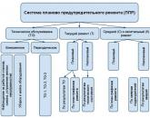

Popular
- Preventive maintenance and its role in production
- Planned preventive maintenance of equipment
- On the procedure for placing non-stationary objects of seasonal trade
- Provisions on the placement of non-stationary shopping facilities
- Decorative painting in kindergarten "magic curl" is a joint activity of the teacher and
- Synopsis of the organization and conduct of classes on cognitive development in the second junior group "Bird feeder
- New professions Where to get information about the right specialists
- Plasticine diplodocus. Sculpting lesson. How to easily make basic shapes from plasticine: a ball, cone, cylinder, plait, brick How to make a cylinder from plasticine
- Rating of recruiting agencies
- Rating of recruiting agencies